Overview
Today we put our tools together (production functions/isoquants and isocost lines) to solve the firm’s cost minimization problem. Again, we do not solve this constrained optimization problem with calculus, but by looking graphically, and using an algebraic rule that should make intuitive sense.
Again, these tools and rules are almost identical to how we solved the consumer’s problem. Compare to or to !, with a major exception:
Consumers:
- choose goods to maximize utility subject to their budget constraint
- budget constraint (line) is what is fixed
- get on highest indifference curve tangent to budget constraint
Producers (Firms):
- choose inputs to minimize cost subject to producing the optimal amount (their constraint)
- isoquant curve is what is fixed (want to produce a specific amount!)
- get on lowest isocost line tangent to isoquant curve
We finally wrap up with a discussion of returns to scale.
Slides
Below, you can find the slides in two formats. Clicking the image will bring you to the html version of the slides in a new tab. Note while in going through the slides, you can type h to see a special list of viewing options, and type o for an outline view of all the slides.
The lower button will allow you to download a PDF version of the slides. I suggest printing the slides beforehand and using them to take additional notes in class (not everything is in the slides)!
Practice
Today we will be working on practice problems. Answers will be posted later on that page.
Problem Set 3 Due Monday March 21
Problem set 3 (on classes 2.1-2.3) is due by the end of the day Monday, March 21 by upload to Blackboard Assignments.
Appendix
A Change in Relative Factor Prices
If an input (labor or capital) changes in price, we saw that it rotated the isocost line by changing the slope, and the intercept for that input. How does it affect the cost-minimizing (optimal) combination of inputs?
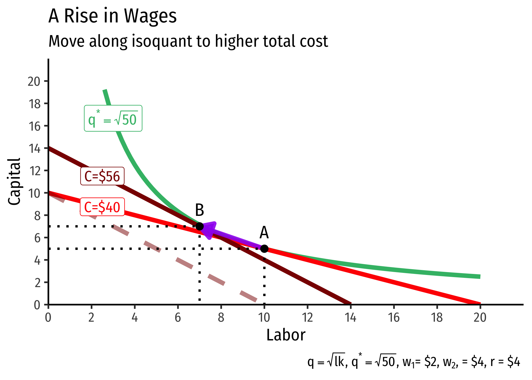
It turns out, a change in one input’s price relative to the other is likely to change the ratio of inputs, as well as the total cost of production due to the mathematics and geometry of cost minimization. Recall the cost-minimizing combination of inputs occurs where the slope of the isoquant is equal to the slope of the lowest isocost line tangent to the isoquant. In the graph below, this occurs at point .
Then, suppose the price of labor increases from 4. This causes a move along the isoquant from to , the firm substitutes more capital for labor, and this costs more!
Why does the optimal isocost line rotate along both axes (i.e. both axis-endpoints change)? With the budget constraint, we saw a change in one price caused the budget constraint to rotate and change an endpoint only along the axis with the good that changed in price.
Here, recall that the isoquant is unmovable - this is the set optimal quantity we want to produce. If an input were to change in price, that would rotate the isocost line and change only the intercept of that input that changed in price, as with a budget constraint. However, that new line (dashed darker red line) would not be tangent to our original budget constraint anymore - that is, we could not produce the output we want at the same total cost as before. Thus, it must be on a new isocost line (indicating a different total cost), just with the same slope as the new isocost line after the price change.
Note you could also go in the other direction. Begin at point and suppose the price of labor decreases (or perhaps the price of capital increases). Then, the firm will substitute more labor for capital, and this will cost less!
Improvements in Technology
We defined our original production function as including an “input” called “total factor productivity.” In our Cobb-Douglas case, we included it in our function as , as in:
Now let’s see how this affects production. Suppose the firm wants to produce 100 units of output at a particular set of input prices, with the following technology (represented by the production function):
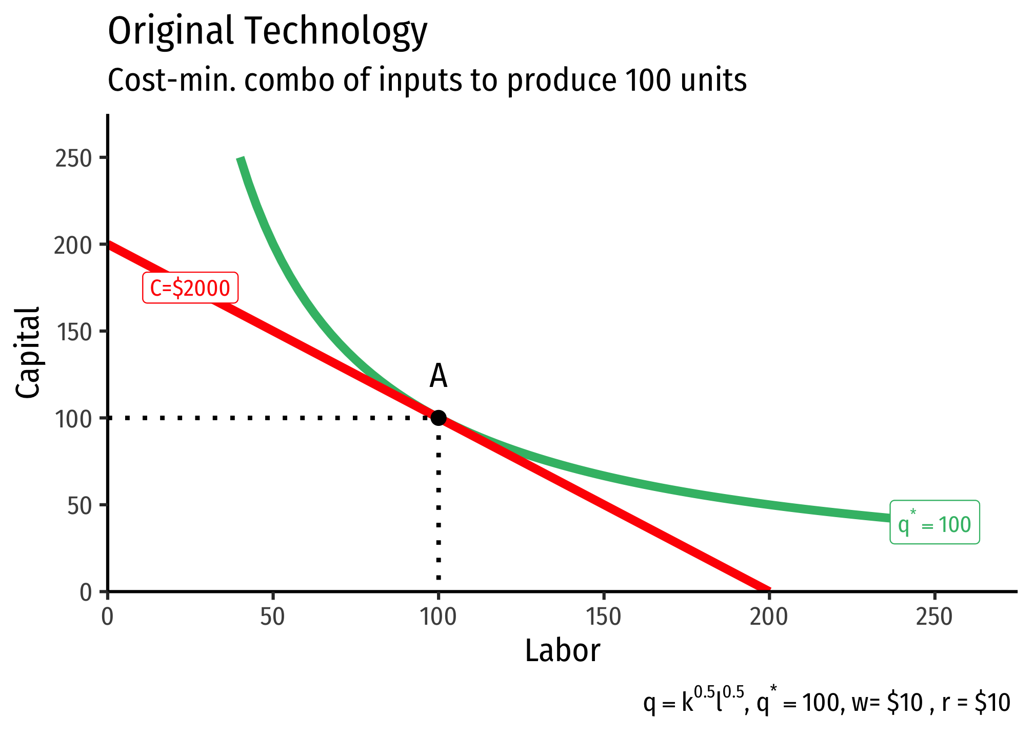
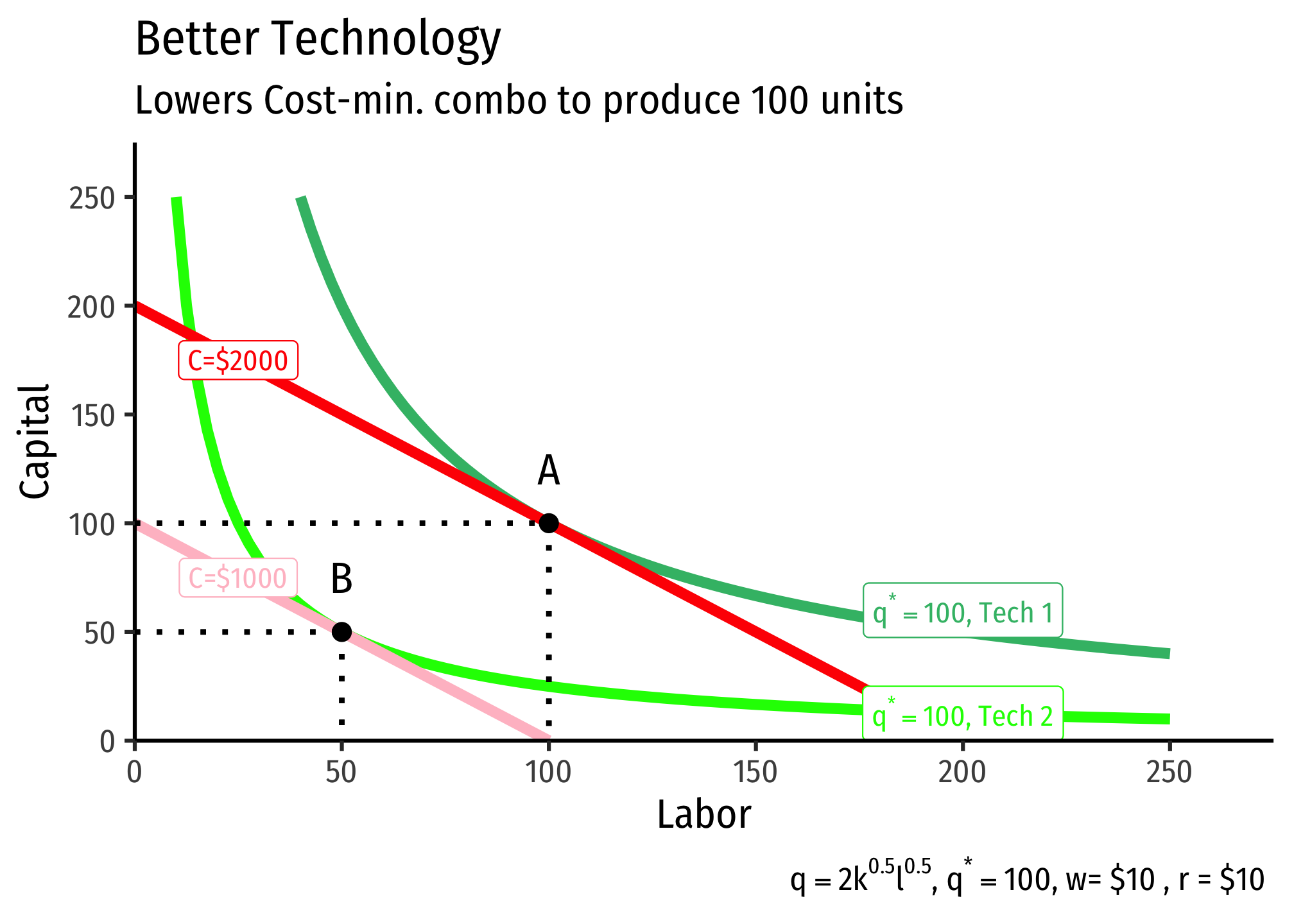
Then the firm’s “technology” improves, such that its new production function is
Notice total factor productivity has doubled, such that, for the same amount of inputs and , the firm can now produce twice as much output . So suppose again the firm still wishes to produce , the same as before. Under the new technology, the firm can produce the same output with fewer inputs. This is the definition of productivity increases or, for an entire economy, economic growth.