Overview
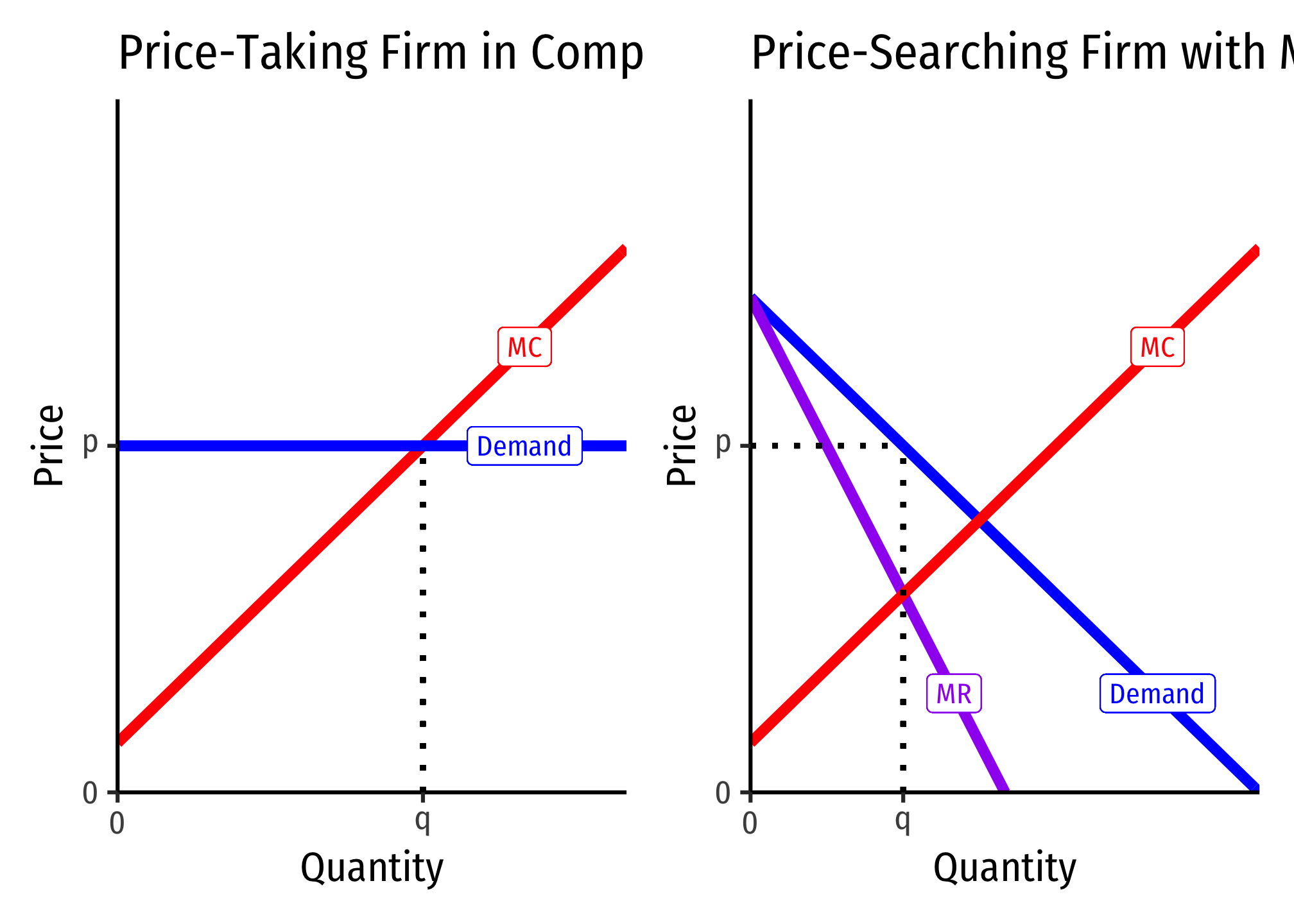
Today we begin our look at “imperfect competition,” where firms have market power, meaning they can charge and search for the profit-maximizing quantity and price. Today is merely about how do change the model to understand how a firm with market power behaves. To assist us, we begin with an extreme case of a single seller, i.e. a monopoly. For now we only assume that there is a single firm, and see how it behaves differently than if it were in a competitive market. Next class we will begin to explore what could cause a market to have only a single seller, and what are some of the social consequences of market power.
Practice
Today we will be working on practice problems. Answers will be posted later on that page.
Slides
Below, you can find the slides in two formats. Clicking the image will bring you to the html version of the slides in a new tab. Note while in going through the slides, you can type h to see a special list of viewing options, and type o for an outline view of all the slides.
The lower button will allow you to download a PDF version of the slides. I suggest printing the slides beforehand and using them to take additional notes in class (not everything is in the slides)!

Assignments
Problem Set 5 Due Wednesday April 27
Problem set 5 (on classes 3.1-3.5) is due by Wednesday, April 27 by PDF upload to Blackboard Assignments. This will be your final graded homework!
Appendix
Monopolists Only Produce Where Demand is Elastic: Proof
Let’s first show the relationship between and price elasticity of demand, .
Remember, we’ve simplified , where because on a demand curve, .
Now that we have this alternate expression for , lets assume and set them equal to one another to maximize profits:
I rearrange the last line only to remind us that is always negative!
Now note the following:
- If , then is negative. Since is assumed to be positive, it cannot equal a negative , hence this is not profit-maximizing.
- If , then is 0. Only if is also 0 is this profit-maximizing.
- If , then is positive. It can equal a positive to be profit-maximizing.
Hence, a monopolist will never produce in the inelastic region of the demand curve (where , and will only produce at the unit elastic part of the demand curve (where if . Thus, it generally produces in the elastic region where .
See the graphs on slide 32.
Derivation of the Lerner Index
Marginal revenue is strongly related to the price elasticity of demand, which is 1
We derived marginal revenue (in the slides) as:
Firms will always maximize profits where:
The left side gives us the fraction of price that is markup , and the right side shows this is inversely related to price elasticity of demand.
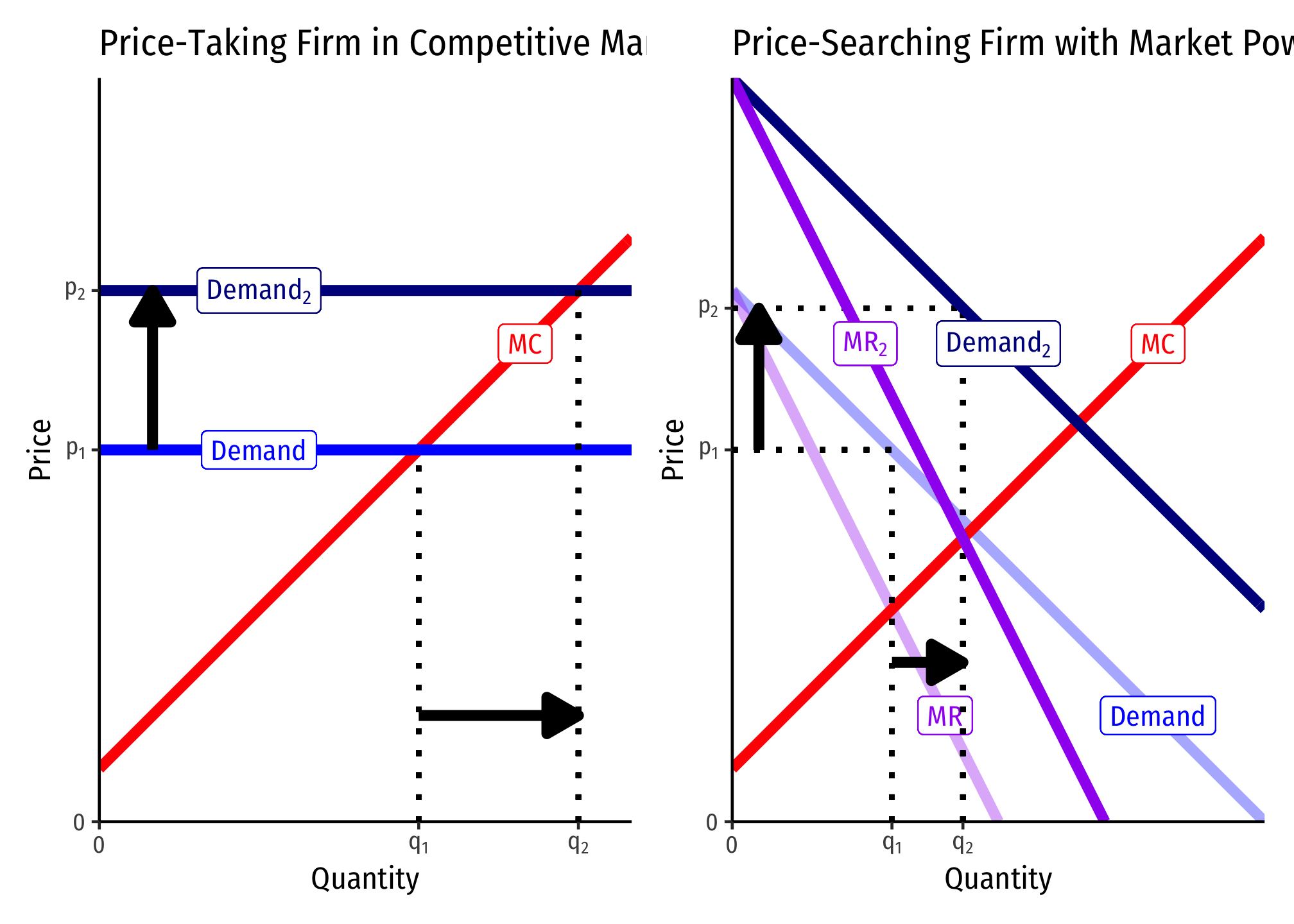
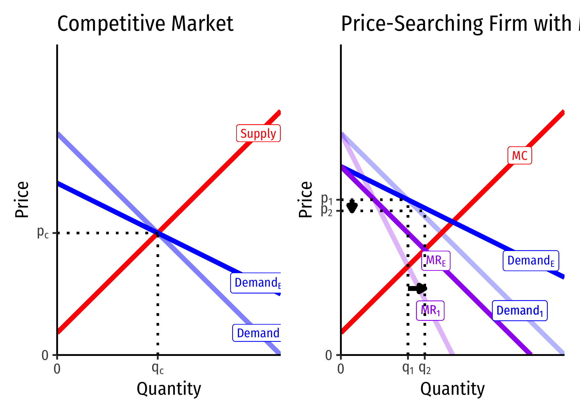
Firms With Market Power vs. Competitive Firms’ Responses to Market Changes
Consider a firm in a competitive market (left) and a firm with market power (right):
An Increase in Firms’ Marginal Cost
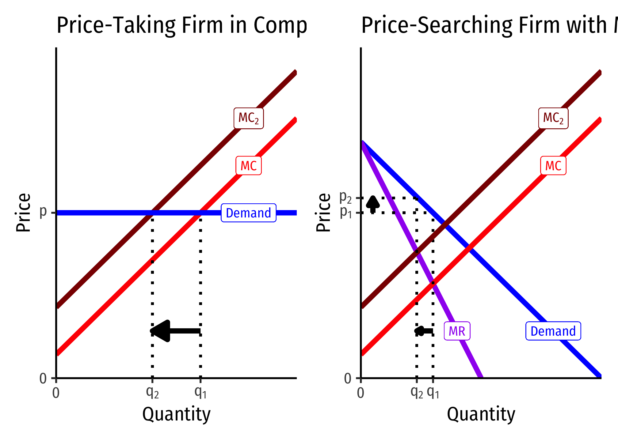
A competitive firm responds by only changing its output (since it cannot control price), whereas the firm with market power changes both its and .
I sometimes simplify it as , where “slope” is the slope of the inverse demand curve (graph), since the slope is .↩︎