Assignments

Problem Set 4 Due Fri Apr 1

Problem set 4 (on classes 2.4-2.6) is due by the end of the day Friday, April 1 by upload to Blackboard Assignments.

Appendix

Common Cost Assumptions

Economists often make simple assumptions about costs to illustrate key concepts without marring the analysis with unnecessary complexity. This also makes graphs quite easy to point to and calculate key areas, such as profits or deadweight losses.

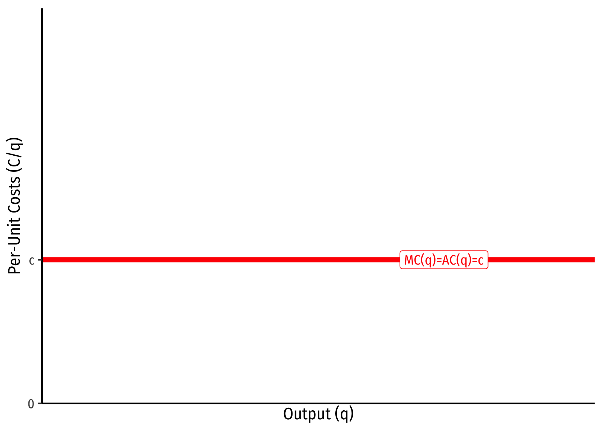
One common set of cost assumptions is the following:

1. A firm has no fixed costs
2. A firm has constant marginal costs, \(MC(q)=c\) where \(c\geq0\)

If this is the case, then we can show that average costs will be equal to marginal costs, i.e. \(MC=AC=AVC=c\).

Since marginal cost is the first derivative of the total cost function, integrating a marginal cost function \(MC=c\) leaves with with a total cost function of \(C(q)=cq\).¹ If this is the case, then we can find the average cost:

\[\begin{align*} C(q)&=cq\\ AC(q)=\frac{C(q)}{q}&=\frac{cq}{q}\\ AC(q)&=c\\ \end{align*}\]

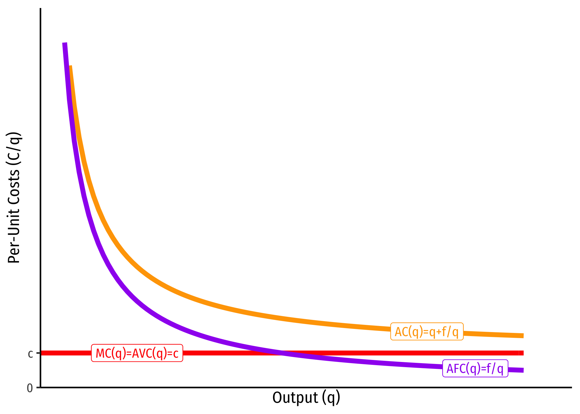
Another common set of cost assumptions is the following:

1. A firm has fixed costs, \(f\)
2. A firm has constant marginal costs, \(MC(q)=c\) where \(c\geq0\)

If this is the case, then we can show that average costs are strictly decreasing over all output \(q\geq0\).

Again, we can integrate marginal cost to the total cost function (but here we need the arbitrary constant from integration, which we shall label \(f\), for fixed costs): \(C(q)=cq+f\). We can then find the average cost:

\[\begin{align*} C(q)&=cq+f\\ AC(q)=\frac{C(q)}{q}&=\frac{cq+f}{q}\\ AC(q)&=c+\frac{f}{q}\\ \end{align*}\]

Since \(f>0\), as \(q \rightarrow \infty\), \(AC(q) \rightarrow c\), that is, average cost is getting asymptotically close to marginal cost, \(c\), but will never intersect it. Note, I also included AFC, which again is always decreasing, and asymptotically approaching 0.

The importance of this type of cost structure is that it creates economies of scale, and represents a lot of industries that tend towards natural monopoly.