Producer Surplus

You may recall from principles of microeconomics the concepts of consumer surplus and producer surplus in markets. While we will study them in our next unit with Supply & Demand, we can talk about the producer surplus to each firm here.

Producer surplus essentially measures the “gains from exchange” to each party — for a producer, it is how much they benefit (on net) from selling their output.

There are three equivalent ways of visualizing and measuring producer surplus for a firm. I will begin with a generalized series of cost curves:

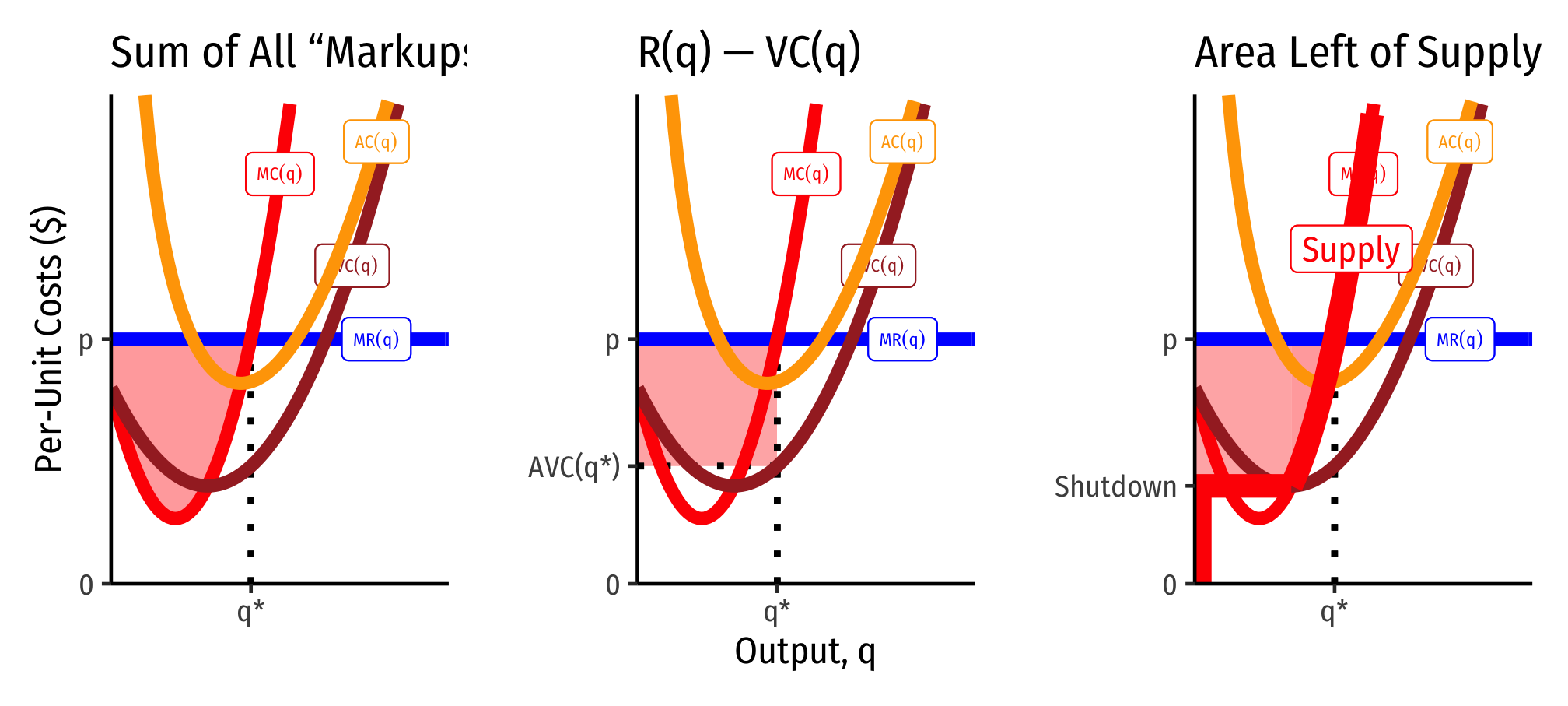
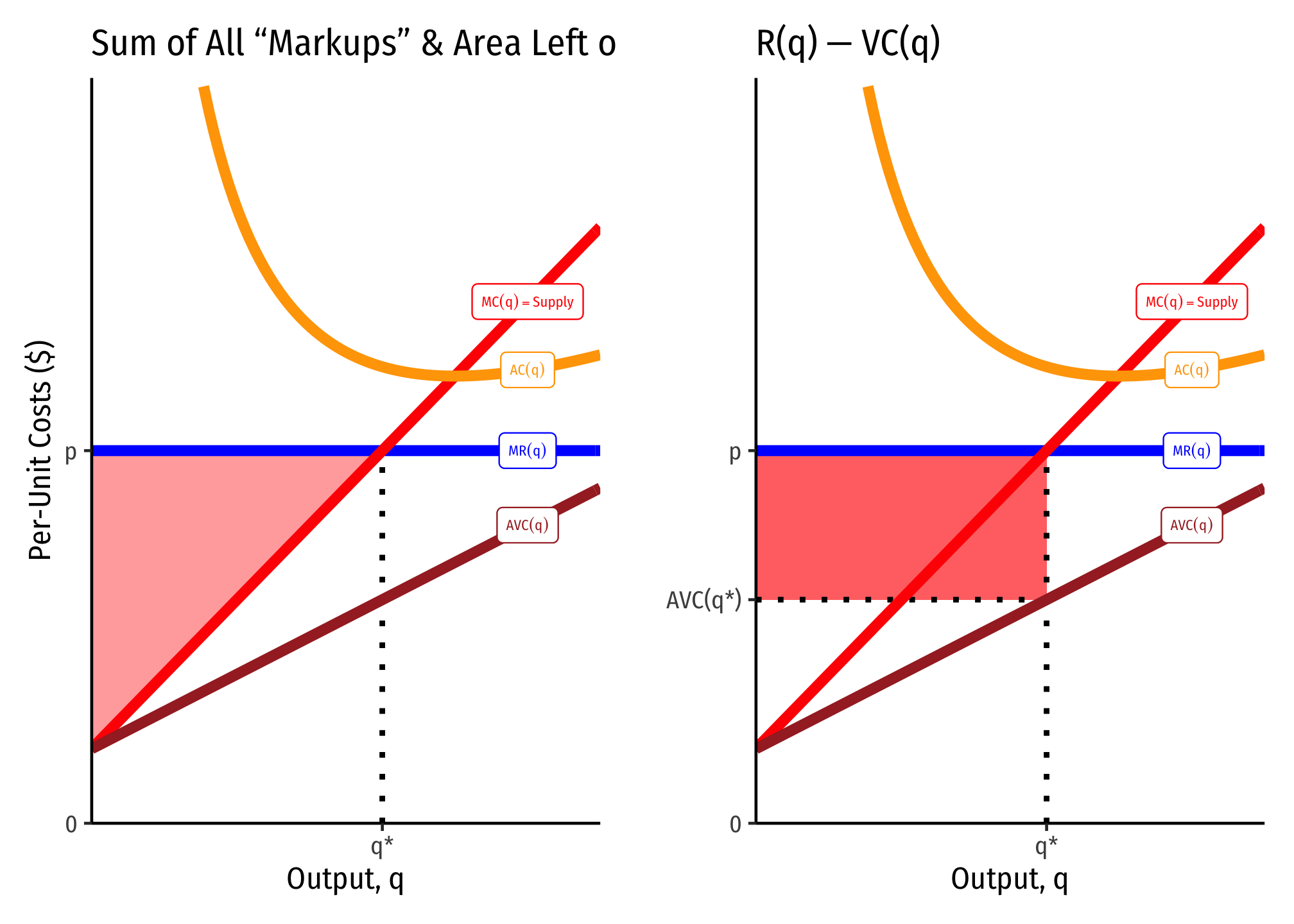
These often converge, and are also easier to identify when marginal cost is linear (and thus, average variable cost is also linear, and starts at the same point as marginal cost, the shutdown price). Here it producer surplus becomes the familiar “triangle” between the market price and the supply curve. Note we can also calculate it as the rectangle of revenues minus variable costs (right).

What’s the Difference Between Producer Surplus and Profit?

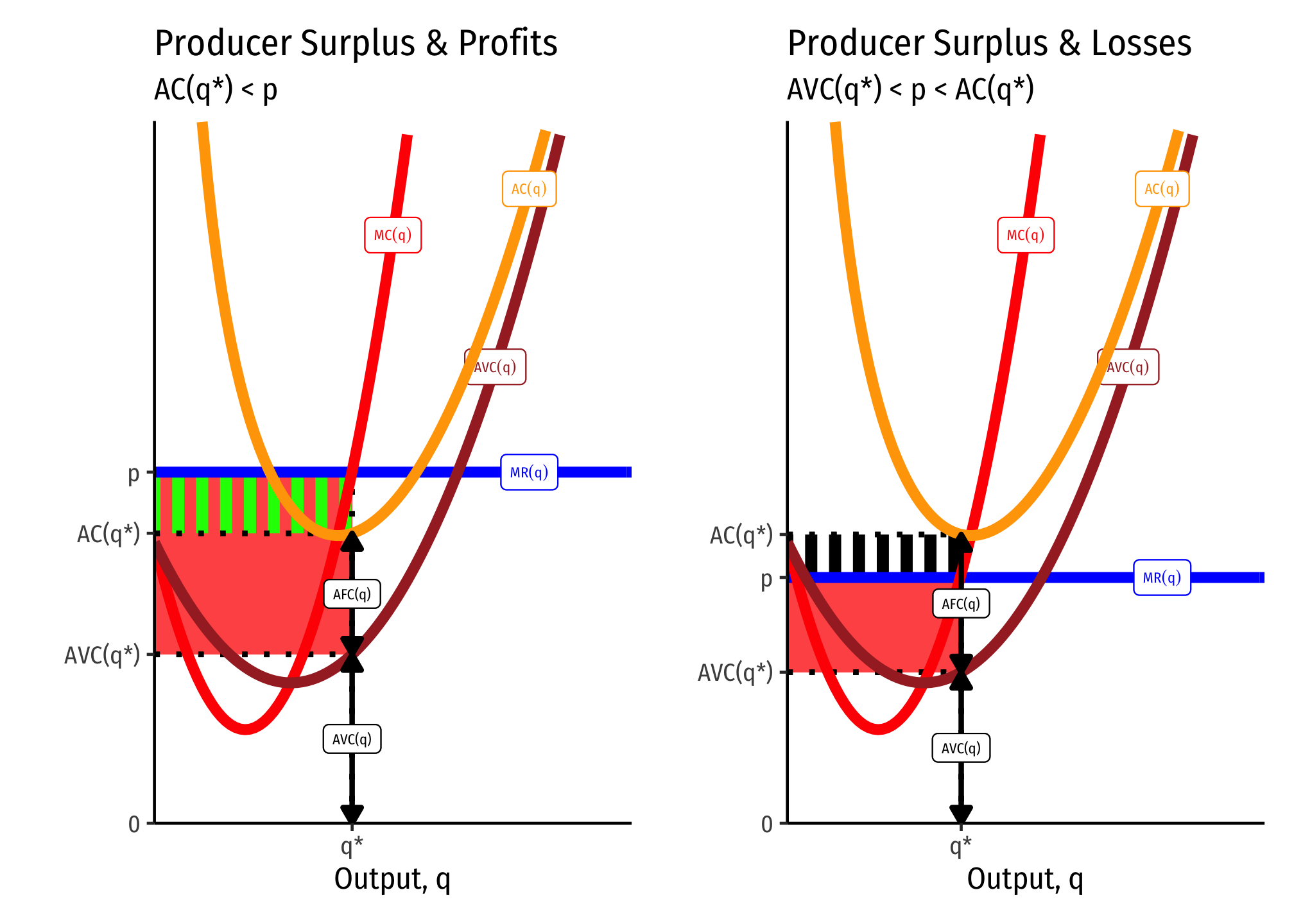
Producer surplus (PS) looks a lot like profits \((\pi)\), but they are in fact different:

\[\begin{align*} \color{red}{PS} &= R(q) - VC\\ & \\ \color{green}{\pi} & = R(q) - C(q) \\ \color{green}{\pi} &= R(q) - VC(q)-f\\ & \\ \color{green}{\pi}-\color{red}{PS}&=-f\\ \color{green}{\pi}&=\color{red}{PS}-f\\ \end{align*}\]

Producer surplus does not include fixed costs \((f)\), but profit \((\pi)\) does.

If there are no fixed costs, then producer surplus and profits are the same thing.

This leads to some other implications connected with the shutdown condition \(p<AVC(q)\). A firm will always earn producer surplus, but may earn losses (negative profit) so long as the price is above the shutdown price. This is because each unit of output sold generates at least enough revenues as (non-fixed) variable costs, \(pq \geq VC(q)\) or (dividing by \(q)\) \(p \geq AVC(q)\).

A firm will shut down production in the short run if it earning no producer surplus. This would happen if it earns fewer revenues than (non-fixed) variable costs: \(pq < VC(q)\) or (dividing by \(q)\) \(p < AVC(q)\).

Thus producer surplus exists \(\iff p>AVC(q)\).

Economic Rents

Economic rents come from factors of production that are fixed in supply (talent, productive land, etc.). Take productive land for a moment, which has a fixed supply. There would be just as much land supplied at a price of zero dollars as at $1000 (its factor supply curve is perfectly inelastic), because (assume for a moment) we can’t produce any more of it.

For the economy as a whole, it is the price of agricultural products that determines the value of agricultural land (used to grow agricultural products). But for the individual farmer (firm producing food), the value of her land that she rents is a cost of production that enters into the pricing of her product.

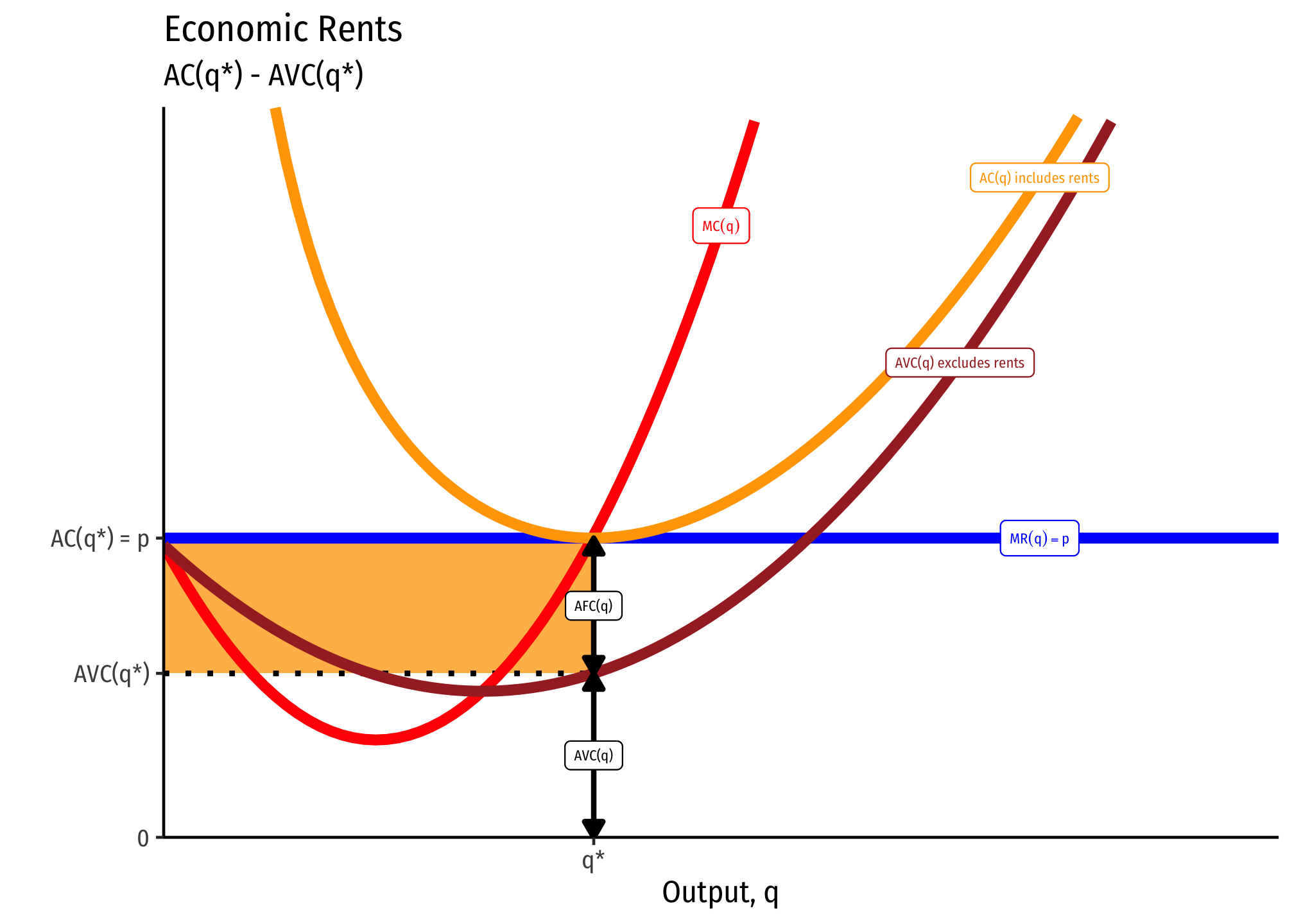
Below, \(AVC(q)\) represents the average cost curve for all variable factors of production, i.e. excluding land costs (the fixed factor). If the price of the crop grown on this land is p∗, then the “profits” attributable to the land are measured by the area in orange: these are the economic rents. This is how much the rent (price) of the land would be in a competitive market — whatever it took to drive the profits to zero.

In long run equilibrium, if there is competition for the productive land, the price of the land will be bid upwards, raising the cost to the farmers who must rent it, and raising the income to the owner of the land. Thus, economic rents increase to push profits to the firms to zero (but higher-than-opportunity-cost returns to the owners of land), since they must pay more to rent it.

The average cost curve including the cost of the land is \(AC(q)\). Since the equilibrium rent for the land will be whatever it takes to drive firm profits to zero:

\[\begin{align*} \underbrace{R(q^\star) - C(q^\star)}_{\pi} &= 0\\ p^\star q^\star - VC(q^\star) - rent &= 0\\ rent &= p^\star q^\star - VC(q^\star)\\ \end{align*}\]

In other words, economic rent is the difference between revenues \((p^\star q^\star)\) and variable costs. On the graph below, this is shaded in orange; we can also see it per unit as the difference between price and average variable costs (i.e. \(AFC(q))\).

This shows that rent is also precisely the same thing as producer surplus (discussed above). That means you can also calculate the economic rent as the area to the left of the marginal cost curve, etc.

Given what we said in the equations above, it is now easier to see the truth of what we said earlier: it is the market equilibrium price that determines economic rents, not the reverse. The firm supplies along its marginal cost curve — which is independent of the cost of the fixed factors. Rents will adjust to drive profits to zero.