2.4 — Costs of Production — Class Content

Monday, March 21, 2021

Problem Set 3 is due by the end of the day today.

Overview

Today we cover costs before we put them together next class with revenues to solve the firm’s (first stage) profit maximization problem. While it seems we are adding quite a bit, and learning some new math problems with calculating costs, we will practice it more next class, when put together with revenues.

Readings

  • Ch. 7 in Goolsbee, Levitt, and Syverson, 2019

Slides

Below, you can find the slides in two formats. Clicking the image will bring you to the html version of the slides in a new tab. Note while in going through the slides, you can type h to see a special list of viewing options, and type o for an outline view of all the slides.

The lower button will allow you to download a PDF version of the slides. I suggest printing the slides beforehand and using them to take additional notes in class (not everything is in the slides)!

2.4-slides

Download as PDF

Assignments

Problem Set 3 Due Mon Mar 21

Problem set 3 (on classes 2.1-2.3) is due by the end of the day Monday, March 21 by upload to Blackboard Assignments.

Appendix

Marginal Cost and Variable Cost

Marginal cost is defined as the change in total costs from a change in output: \[MC(q)=\frac{\Delta C(q)}{\Delta q}\]

Recall that total cost is the sum of fixed and variable costs

\[C(q)=f+VC(q)\] However, since fixed costs never change, any change in total cost is a change in variable cost \[\Delta C(q) = \Delta VC(q)\]

Thus, marginal cost actually measures the change in variable costs from a change in output: \[MC(q)=\frac{\Delta C(q)}{\Delta q}=\frac{\Delta VC(q)}{\Delta q}\] Thus, fixed cost has no effect on marginal cost, and marginal cost is always measuring the change in variable costs with additional output.

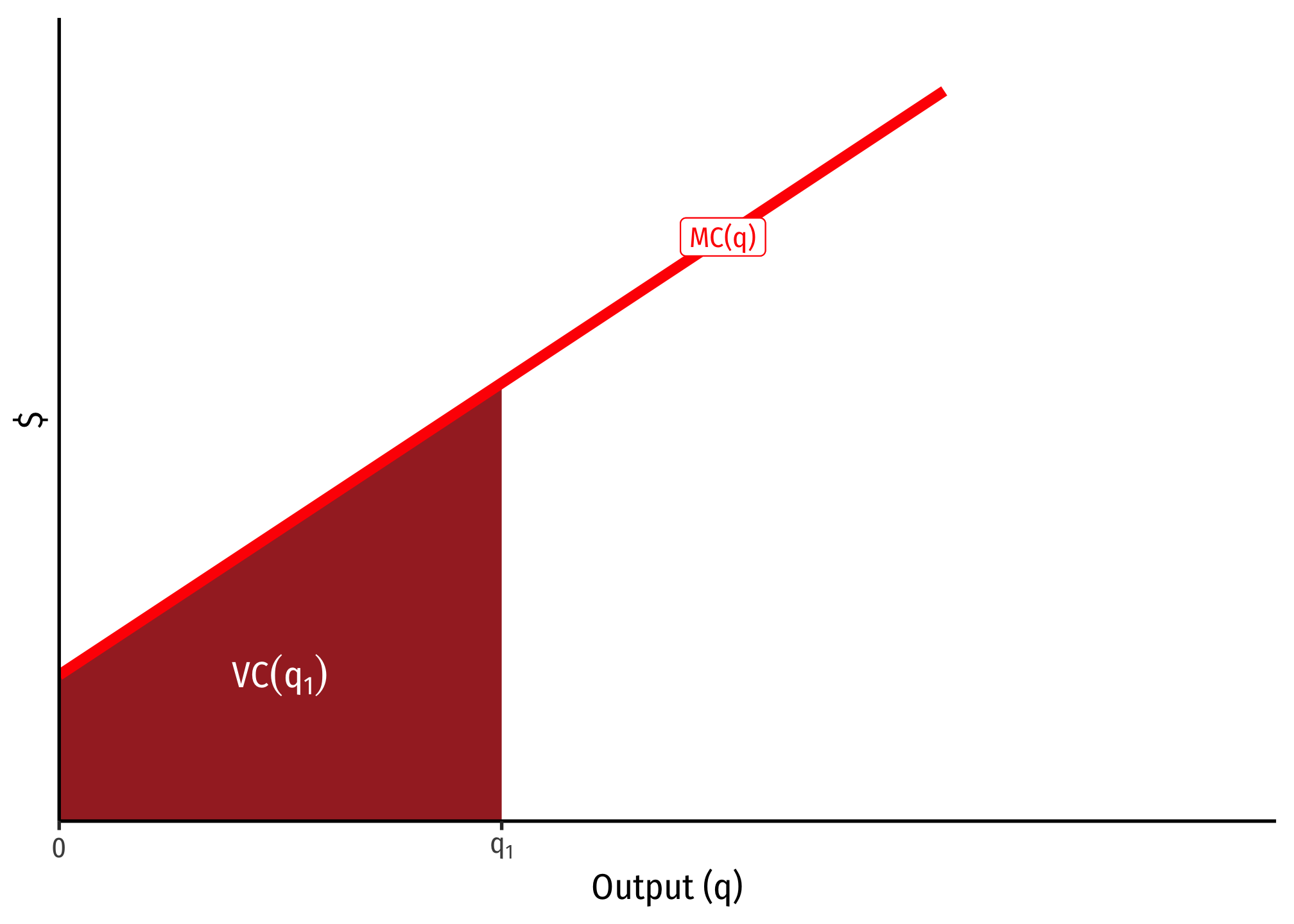
Furthermore, because of this relationship with marginal cost measuring the change in variable cost from additional output, for any specific quantity of output, e.g. \(q_1\), the variable cost of producing \(q_1\) can be seen on the graph below as the total area under the marginal cost curve to the left of \(q_1\):

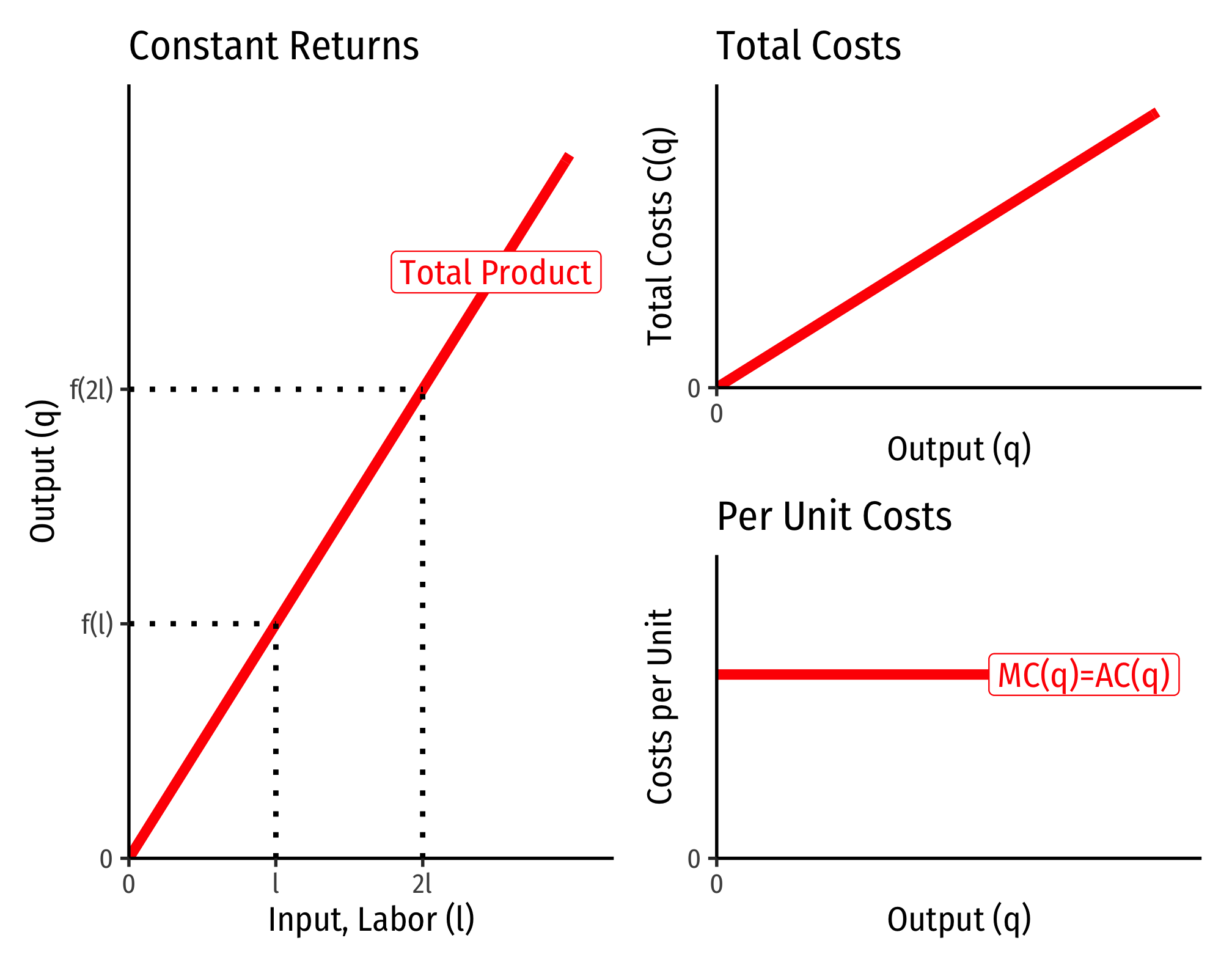
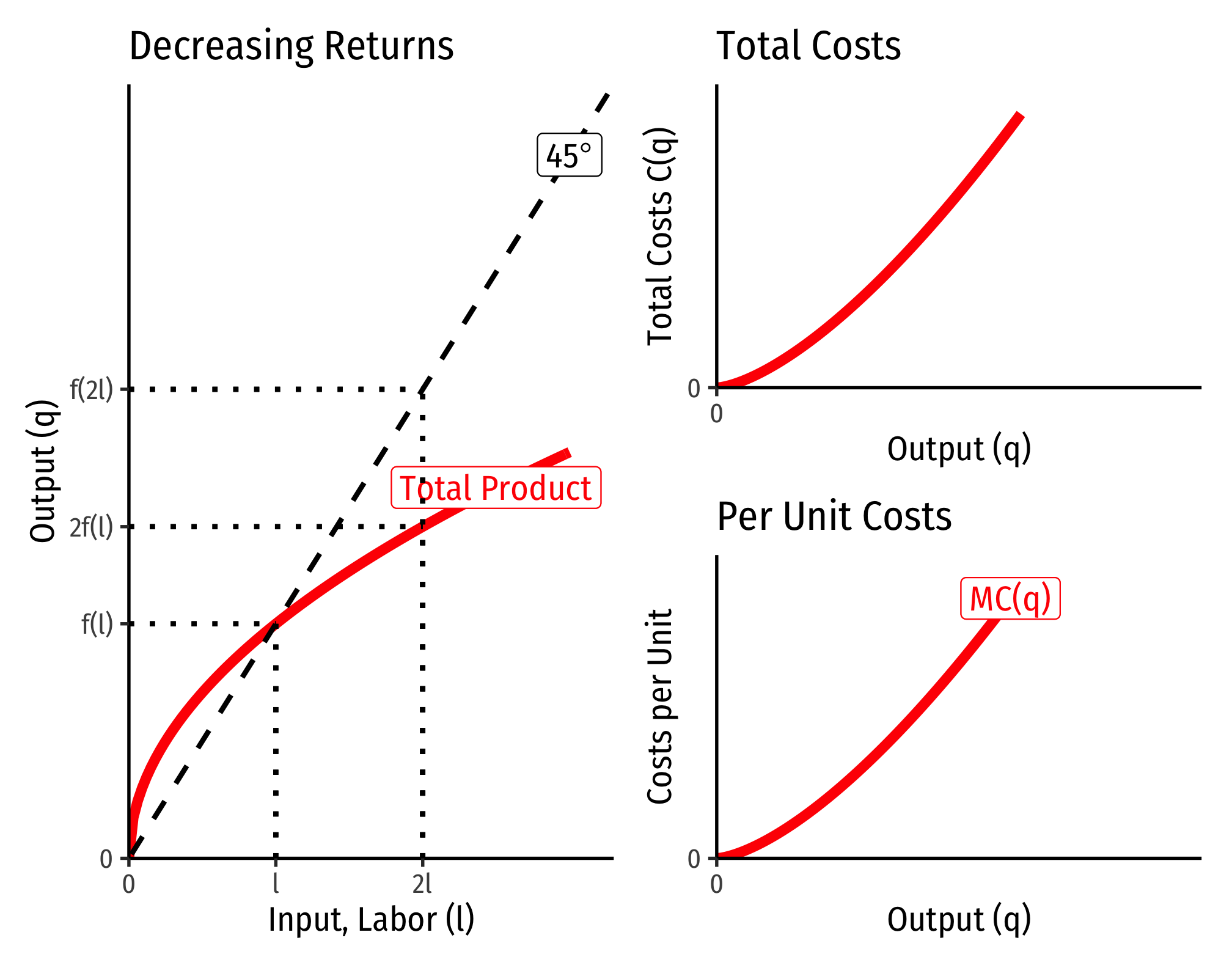
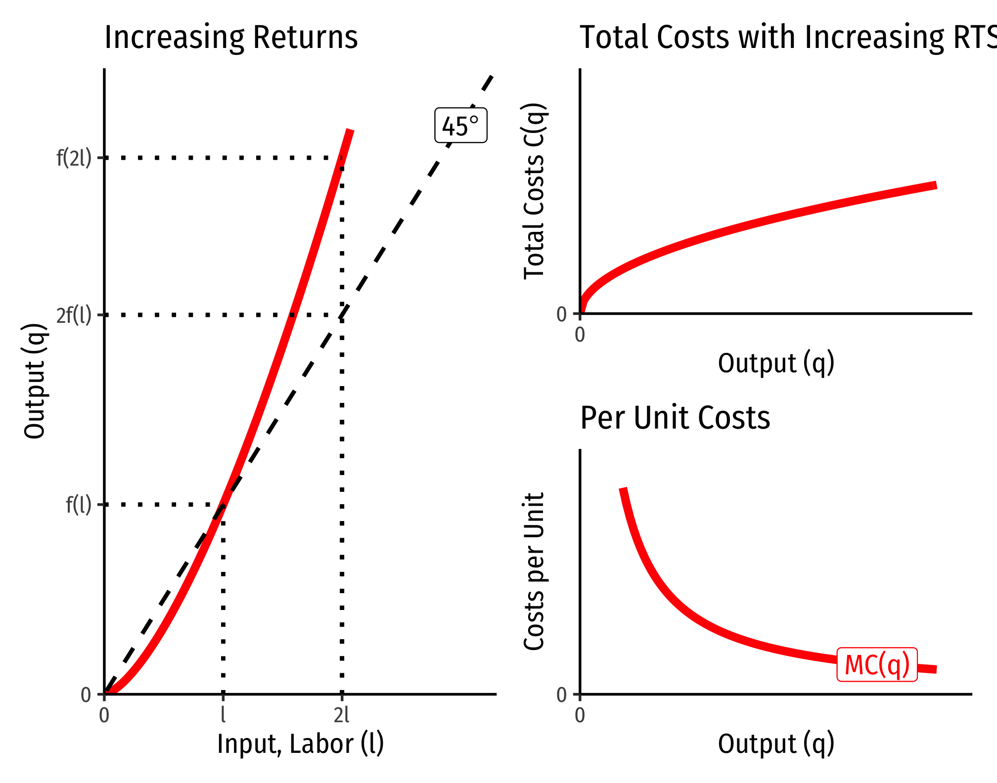
The Relationship Between Returns to Scale and Costs

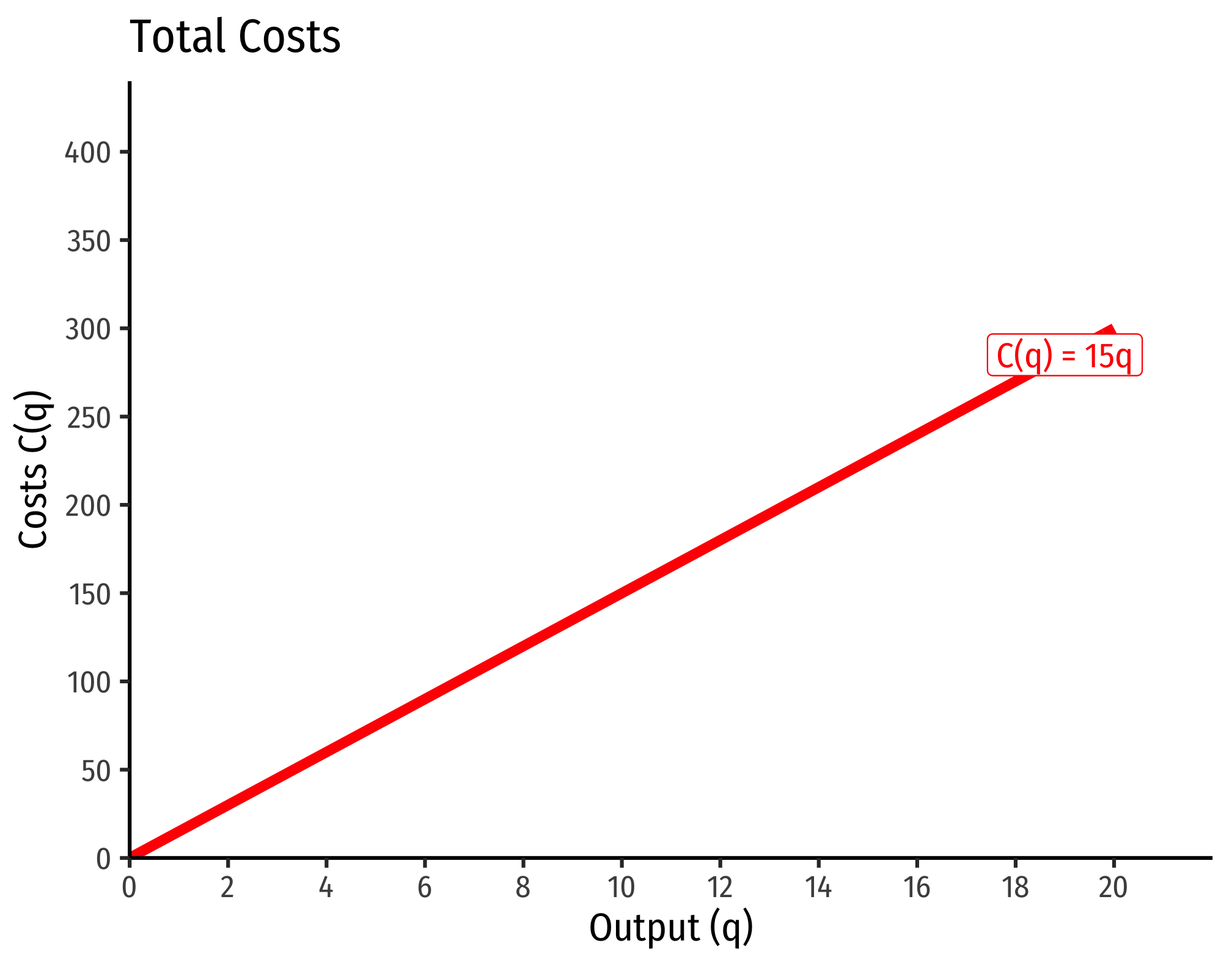
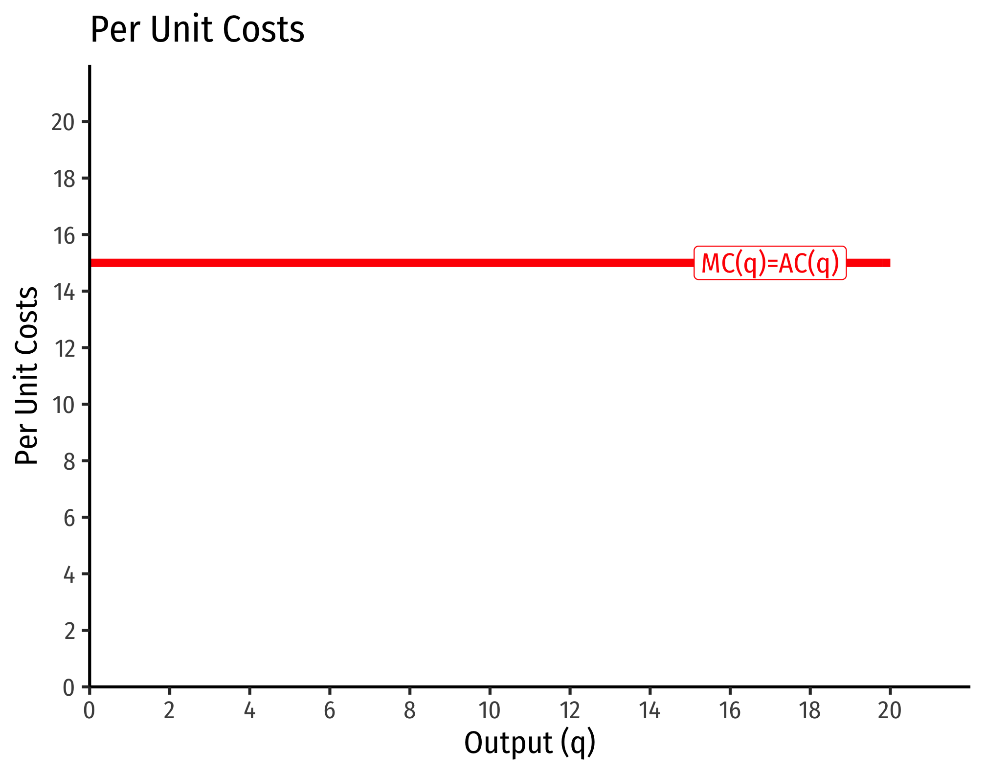
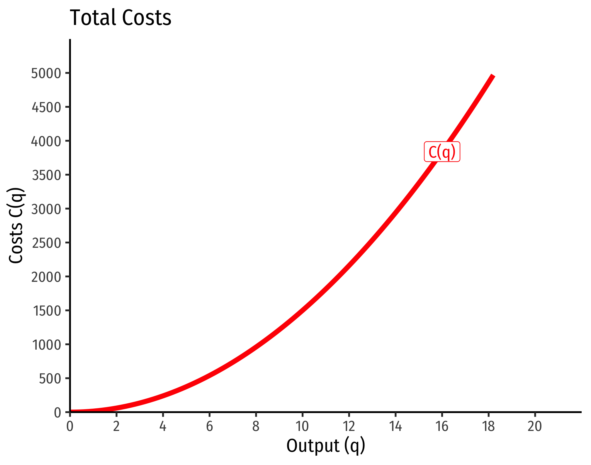
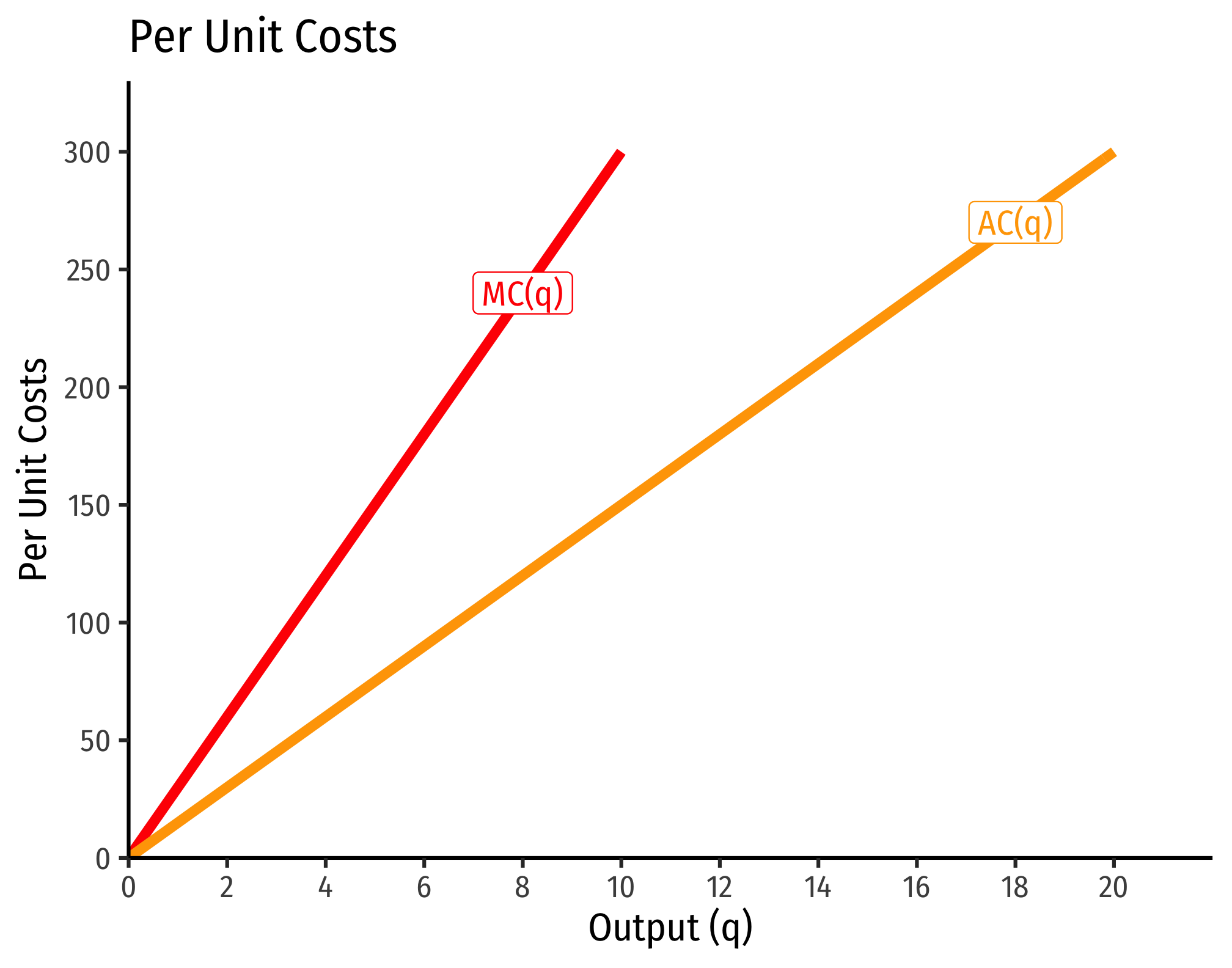
There is a direct relationship between a technology’s returns to scale1 and its cost structure: the rate at which its total costs increase2 and its marginal costs change3. This is easiest to see for a single input, such as our assumptions of the short run (where firms can change \(l\) but not \(\bar{k})\):

\[q=f(\bar{k},l)\]

Constant Returns to Scale:

Decreasing Returns to Scale

Increasing Returns to Scale

Cobb-Douglas Cost Functions

The total cost function for Cobb-Douglas production functions of the form \[q=l^{\alpha}k^{\beta}\] can be shown with some very tedious algebra to be:

\[C(w,r,q)=\left[\left(\frac{\alpha}{\beta}\right)^{\frac{\beta}{\alpha+\beta}} + \left(\frac{\alpha}{\beta}\right)^{\frac{-\alpha}{\alpha+\beta}}\right] w^{\frac{\alpha}{\alpha+\beta}} r^{\frac{\beta}{\alpha+\beta}} q^{\frac{1}{\alpha+\beta}}\]

If you take the first derivative of this (to get marginal cost), it is:

\[\frac{\partial C(w,r,q)}{\partial q}= MC(q) = \frac{1}{\alpha+\beta} \left(w^{\frac{\alpha}{\alpha+\beta}} r^{\frac{\beta}{\alpha+\beta}}\right) q^{\left(\frac{1}{\alpha+\beta}\right)-1}\]

How does marginal cost change with increased output? Take the second derivative:

\[\frac{\partial^2 C(w,r,q)}{\partial q^2}= \frac{1}{\alpha+\beta} \left(\frac{1}{\alpha+\beta} -1 \right) \left(w^{\frac{\alpha}{\alpha+\beta}} r^{\frac{\beta}{\alpha+\beta}}\right) q^{\left(\frac{1}{\alpha+\beta}\right)-2}\]

Three possible cases:

  1. If \(\frac{1}{\alpha+\beta} > 1\), this is positive \(\implies\) decreasing returns to scale
  • Production function exponents \(\alpha+\beta < 1\)
  1. If \(\frac{1}{\alpha+\beta} < 1\), this is negative \(\implies\) increasing returns to scale
  • Production function exponents \(\alpha+\beta > 1\)
  1. If \(\frac{1}{\alpha+\beta} = 1\), this is constant \(\implies\) constant returns to scale
  • Production function exponents\(\alpha+\beta = 1\)

Example (Constant Returns)

Let \(q=l^{0.5}k^{0.5}\).

\[\begin{align*} C(w,r,q)&=\left[\left(\frac{0.5}{0.5}\right)^{\frac{0.5}{0.5+0.5}} + \left(\frac{0.5}{0.5}\right)^{\frac{-0.5}{0.5+0.5}}\right] w^{\frac{0.5}{0.5+0.5}} r^{\frac{0.5}{0.5+0.5}} q^{\frac{1}{0.5+0.5}}\\ C(w,r,q)&= \left[1^{0.5}+1^{-0.5} \right]w^{0.5}r^{0.5}q^{0.5}\\ C(w,r,q)&= w^{0.5}r^{0.5}q^{1}\\ \end{align*}\]

Consider input prices of \(w=\$9\) and \(r=\$25\):

\[\begin{align*}C(w=9,r=25,q)&=9^{0.5}25^{0.5}q \\ & =3*5*q\\ & =15q\\\end{align*}\]

That is, total costs (at those given input prices, and technology) is equal to 15 times the output level, \(q\):

Marginal costs would be

\[MC(q) = \frac{\partial C(q)}{\partial q} = 15\]

Average costs would be

\[MC(q) = \frac{C(q)}{q} = \frac{15q}{q} = 15\]

Example (Decreasing Returns)

Let \(q=l^{0.25}k^{0.25}\).

\[\begin{align*} C(w,r,q)&=\left[\left(\frac{0.25}{0.25}\right)^{\frac{0.25}{0.25+0.25}} + \left(\frac{0.25}{0.25}\right)^{\frac{-0.25}{0.25+0.25}}\right] w^{\frac{0.25}{0.25+0.25}} r^{\frac{0.25}{0.25+0.25}} q^{\frac{1}{0.25+0.25}}\\ C(w,r,q)&= \left[1^{0.5}+1^{-0.5} \right]w^{0.5}r^{0.5}q^{2}\\ C(w,r,q)&= w^{0.5}r^{0.5}q^{2}\\ \end{align*}\]

If \(w=9\), \(r=25\):

\[\begin{align*}C(w=9,r=25,q)&=9^{0.5}25^{0.5}q^2 \\ & =3*5*q^2\\ & =15q^2\\\end{align*}\]

Marginal costs would be

\[MC(q) = \frac{\partial C(q)}{\partial q} = 30q\]

Average costs would be

\[AC(q) = \frac{C(q)}{q} = \frac{15q^2}{q} = 15q\]


  1. Increasing, decreasing, or constant↩︎

  2. At a decreasing rate, at an increasing rate, or at a constant rate, respectively↩︎

  3. Decreasing, increasing, or constant, respectively↩︎

Previous
Next