Below, find the link to the Math Review guide in PDF format.
If time permits, I will make these into individual pages here on the Resources section.
1 Functions and Inverse Functions
A function is simply a rule that assigns a unique value of a dependent variable (e.g. \(f(x)\)) to each value of an independent variable (e.g. \(x\)): \(x \rightarrow f(x)\)
- Something is not a function if it assigns multiple values of \(y\) for the same value of \(x\) (e.g. on a graph, a vertical line)
- We can relate any independent variable (e.g. \(x\)) to any dependent variable (e.g. \(y\)) so get comfortable using variables other than \(x\) and \(y\)!
In its general form a function can be written as:
\[q = q(p)\]
- “Quantity (\(q\)) is a function of price (\(p\))”
- This expresses that there is a relationship between \(q\) and \(p\), it doesn’t tell us the specific form of that relationship
- \(q\) is the dependent or “endogenous” variable, its value is determined by \(p\)
- \(p\) is the independent or “exogenous” variable, its value is given and not dependent on other variables
- The specific form of this function might be:
\[q = 100-6p\]
- The numbers 100 and 6 are known as parameters, they are parts of the quantitative relationship between quantity and price (the variables) that do not change
- If we have values of \(p\), we can find the value of \(q(p)\):
- When \(p=10\) \[ \begin{align*} q(p)&=100-6p\\ q(10)&=100-6(10)\\ q(10)&=100-60\\ q(10)&=40\\ \end{align*} \]
- When \(p=5\): \[ \begin{align*} q(p)&=100-6p\\ q(5)&=100-6(5)\\ q(5)&=100-30\\ q(5)&=70\\ \end{align*} \]
Multivariate functions have multiple independent variables, such as:
\[q=f(k,l)\]
“Output (\(q\)) is a function of both capital (\(k\)) and labor (\(l\))”
In economics, we often restrict the domain and range of functions to positive real numbers, \(\mathbb{R}_+\), since prices and quantities are never negative in the real world
- Domain: the set of \(x\)-values
- Range: the set of \(y\)-values determined by the function
1.1 Inverse Functions
- Many functions have a useful inverse, where we switch the independent variable and dependent variable
- For example, if we have the demand function: \[q=100-6p\] we may want find the inverse demand function, an equation where \(p\) is the dependent variable, rather than \(q\) (this is how we normally graph Supply and Demand functions!)
- To do this, we need to solve the above equation for \(p\): \[ \begin{align*} q&=100-6p &&\text{The original equation}\\ q+6p&=100 && \text{Add } 6p \text{ to both sides}\\ 6p&=100-q && \text{Subtract } q \text{ from both sides}\\ p&=\frac{100}{6}-\frac{1}{6}q && \text{Divide both sides by 6}\\ \end{align*} \]
1.2 Functions with Fractions
- Many people are rusty on a few useful algebra rules we will need, one being how to deal with fractions in equations
- To get rid of a fraction, multiply both sides of the equation by the fraction’s reciprocal (swap the numerator and denominator), which will yield just 1 \[ \begin{align*} 100&=\frac{1}{4}x & & \text{The equation to be solved for} x\\ \frac{4}{1} \big(\frac{100}{1}\big) &=\frac{4}{1}\bigg(\frac{1}{4}x\bigg) && \text{Multiplying by the reciprocal of } \frac{1}{4} \text{, which is } \frac{4}{1} \\ \frac{400}{1}&=\frac{4}{4}x & & \text{Cross multiplying fractions}\\ 400 & = x & & \text{Simplifying}\\ \end{align*} \]
- Alternatively (if possible), re-imagining the fraction as a decimal may help: \[ \begin{align*} 100&=\frac{1}{4}x && \text{The original equation}\\ 100&=0.25x && \text{Converting to a decimal}\\ 400 & = x && \text{Dividing both sides by }0.25\\ \end{align*} \]
- Add fractions by finding a common denominator: \[ \begin{align*} \frac{4}{3} &+ \frac{2}{5}\\ \bigg(\frac{4 \times 5}{3 \times 5}\bigg) &+ \bigg(\frac{2 \times 3}{5 \times 3}\bigg)\\ \frac{20}{15}&+\frac{6}{15}\\ &= \frac{26}{15}\\ \end{align*} \]
- Multiply fractions straight across the numerator and denominator \[ \frac{4}{3} \times \frac{2}{5}=\frac{4 \times 2}{3 \times 5}=\frac{8}{15} \]
2 Graphing Linear Functions
2.1 Slope-Intercept Form
- A linear function of two variables can be written in slope-intercept form:
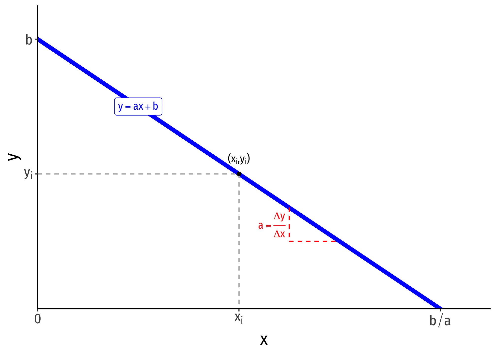
\[y=ax+b\]
- \(y\) is the dependent variable (on the vertical axis)
- \(x\) is the independent variable (on the horizontal axis)
- \(a\) is the slope of the line
- \(a = \frac{\text{rise}}{\text{run}} = \frac{\text{change in }y}{\text{change in }x} = \frac{\Delta x}{\Delta y}\)
- you may have been taught the slope as “\(m\)”, this is just personal taste, but again, get used to using different letters!
- \(b\) is the vertical-intercept, a constant number where the line crosses the vertical axis
- if \(y\) is the dependent variable, this is the “\(y\)-intercept”, \(y\) where \(x=0\)
- Any point on the line has an \(x\)-coordinate and \(y\)-coordinate \((x_i,y_i)\)
2.2 Other Forms
- A linear function can equivalently be expressed in the following form:
\[a_1x_1+a_2x_2=c\]
- \(x_2\) is the dependent variable (on the vertical axis)
- \(x_1\) is the independent variable (on the horizontal axis)
- \(c\) is a constant
- This is a valid equation, but is difficult to visualize in the traditional graph as above. Simply solve for the dependent variable on the vertical axis \((x_2\) as if you were solving for \(y)\):
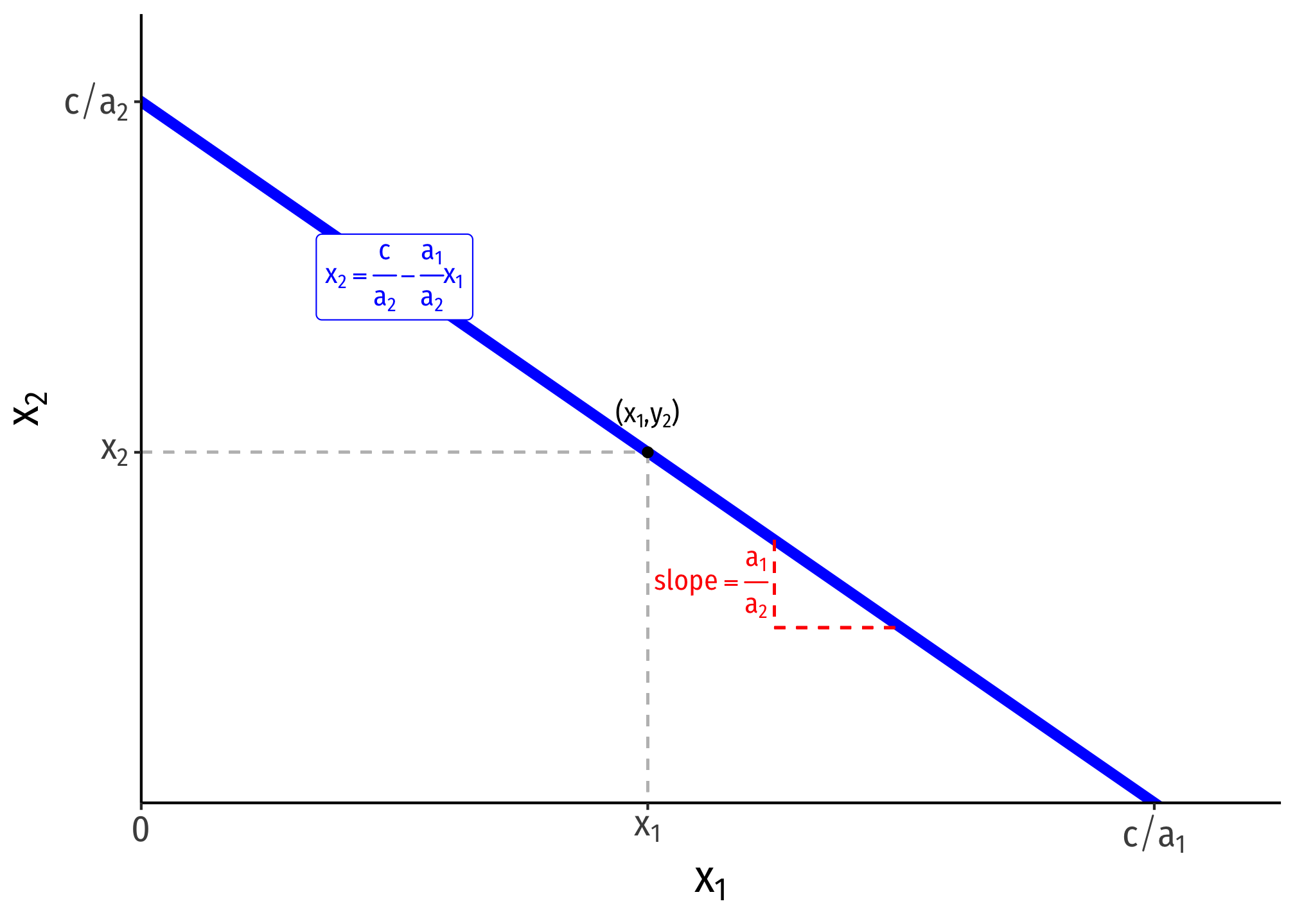
\[\begin{align*} a_1x_1+a_2x_2=c && \text{Original}\\ a_2x_2=c-a_1x_1 && \text{Subtracting }x_1 \text{ term}\\ x_2 = \frac{c}{a_2}-\frac{a_1}{a_2}x_1 && \text{Dividing by }a_2 \\ \end{align*}\]
The vertical intercept is \(\frac{c}{a_2}\)
The horizontal intercept is \(\frac{c}{a_1}\)
The slope is \(-\frac{a_1}{a_2}\)
This is extremely useful for dealing with constraints in constrained optimization problems: budget constraints and isocost lines
2.3 Drawing a Graph From an Equation
If we already have a linear equation that we would like to graph, we can follow these steps:
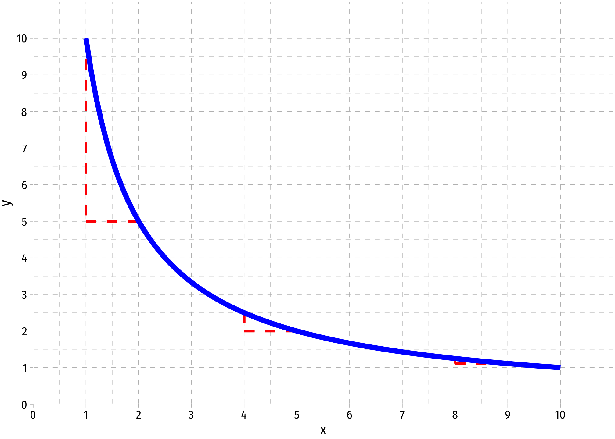
- Take the equation and plug in two values, e.g. if we have:
\[p = \frac{1}{2}q + 4\]
We can find two points on the graph. The easiest one to find is the vertical-intercept, where the line crosses the vertical axis, where \(q=0\), so plug in \(q=0\): \[ \begin{align*} p &= \frac{1}{2}(0)+4\\ p &= 4 \\ \end{align*} \] Thus, one point is \((0,4)\). Note that the constant in the function itself is the \(p-intercept\)! So one valid point will always be \((0,b)\)!
For our second point, let’s plug in \(q=2\): \[ \begin{align*} p &= \frac{1}{2}(2)+4\\ p &= 5 \\ \end{align*} \] Thus, another point is \((2,5)\)
Now, plot the two points on the graph, and connect them with a line
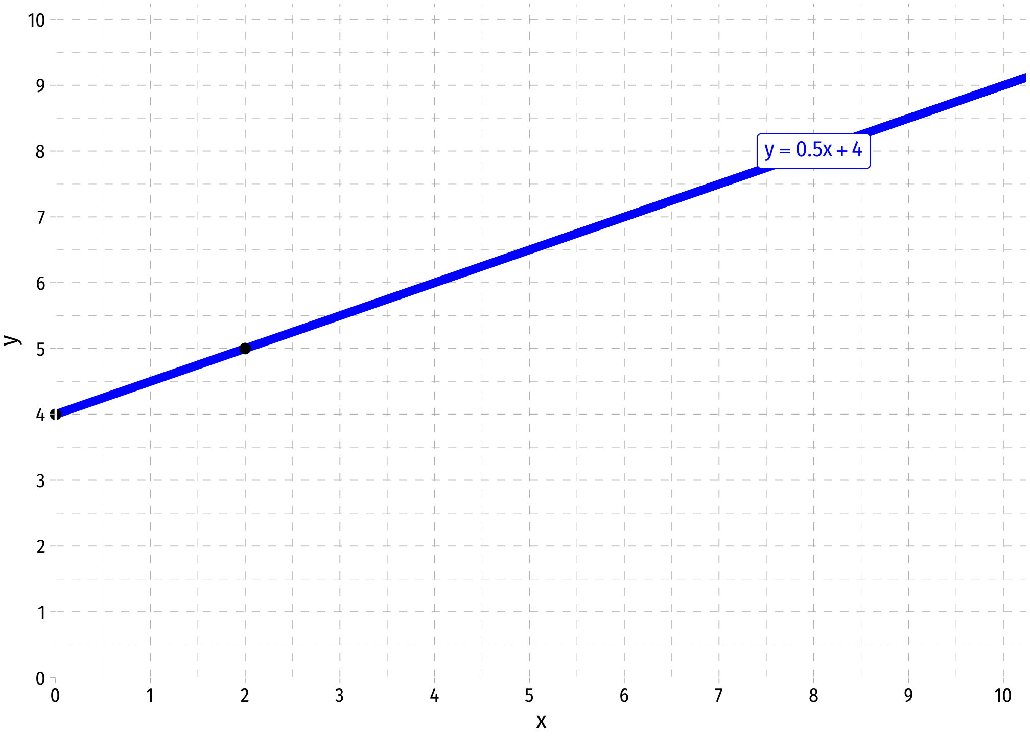
Note: A quick shortcut to plot a line is to find the vertical intercept and plot that, and then find the next point using the slope. Here, start our line at 4 on the vertical axis, and then, as the slope is \(\frac{1}{2}\), for every one unit increase in \(q\), \(p\) increases by \(\frac{1}{2}\). Our second point, (2,5), is a 2 unit increase in \(q\) resulting in a \(1\) unit increase in \(p\).
2.4 Finding an Equation from a Graph
 In order to find the equation of an existing line, we follow these steps:
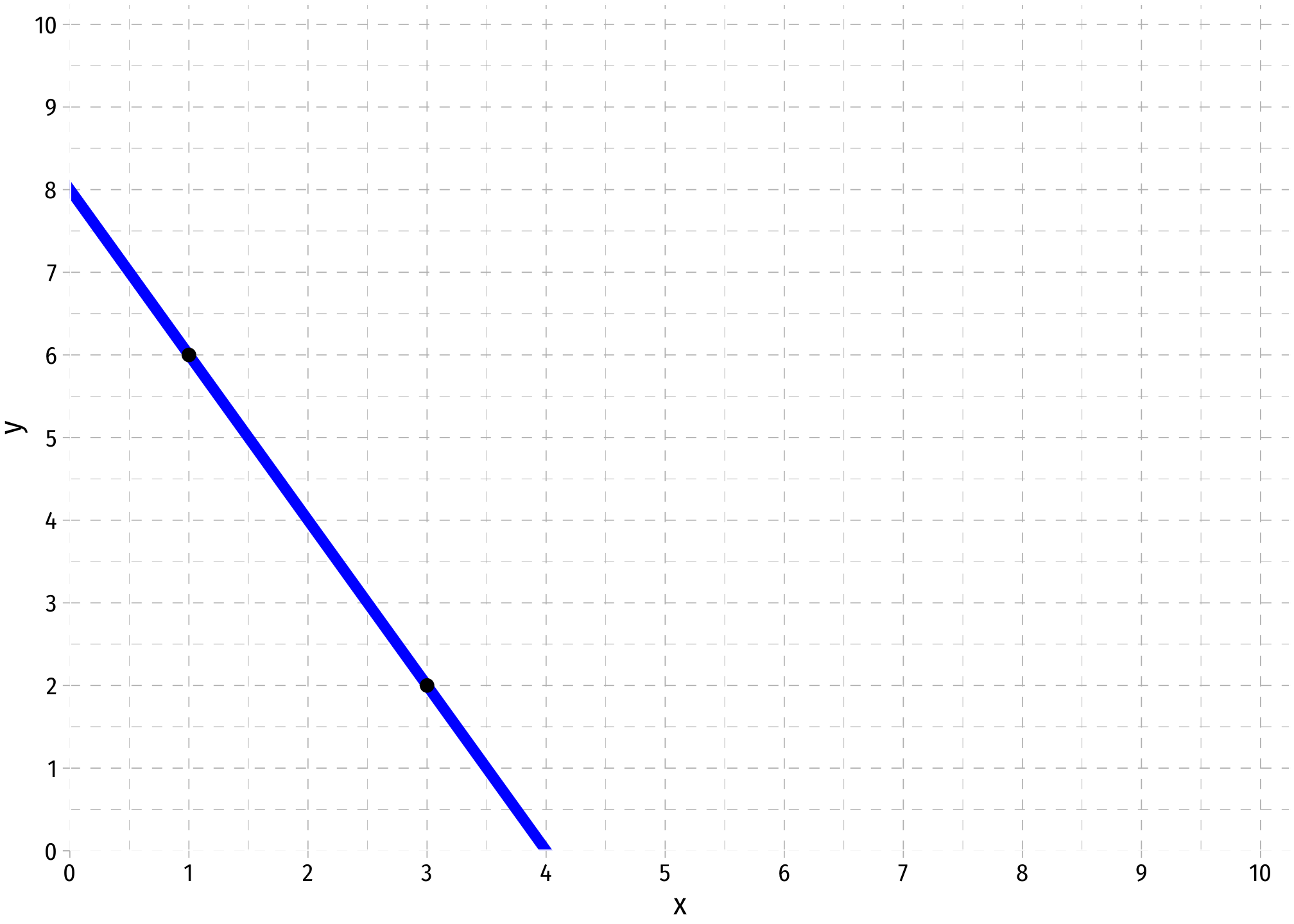
- First, take two points on the line and find the slope, \(a\), between them. Let’s pick \((1,6)\) and \((3,2)\). \[ \begin{align*} \text{Slope} &= \frac{rise}{run} \\ &= \frac{(p_2-p_1)}{(q_2-q_1)}\\ &= \frac{(2-6)}{(3-1)}\\ &= \frac{-4}{2}\\ &= -2\\ \end{align*} \]
There is a shortcut that we can use to find the slope faster by eye-balling the graph: When \(q\) changes by 1, how many units does \(p\) change? If we move from (1,6) to (2,5), \(q\) increases by 1, but \(p\) falls by 2. So the slope is \(-2\). For every one unit increase in \(q\), \(p\) changes by -2.
Now with the slope, we need to find the vertical intercept, or \(b\), we solve this by plugging in the slope and any point on the graph, we will use (1,6): \[\begin{align*} p &= aq+b\\ (6) &= -2(1)+b\\ 6 &= -2+b\\ 8 &= b\\ \end{align*} \] Note, there is another easy way to eye-ball what this value is. It is simply that \(p\) value where \(q=0\), or at what \(p\) value the graph crosses the vertical axis. We can see it is at 8.
Thus, we have the slope and the intercept, so our equation is: \[ p = -2q+8 \]
3 Rates of Change
If \(y\) changes from \(y_1 \rightarrow y_2\), the difference, \(\Delta y = y_2-y_1\)
- \(\Delta y\) is shorthand that means “change in \(y\)”, NOT \(\Delta * y\) (it’s not an entity itself)
- In calculus, the change in \(y\) is often written formally as \(dy\)
We can express the relative difference, comparing the difference with the original value of \(y_1\) as: \[\text{relative change in y}=\frac{y_2-y_1}{y_1}=\frac{\Delta y}{y_1} \]
- e.g. if \(y_1=3\) and \(y_2=3.02\), then the relative change in \(y\) is: \[\frac{y_2-y_1}{y_1}=\frac{3.02-3}{3}=0.0067\]
It’s most common to talk about the percentage change in \(y\) (\(\% \Delta y\)), also called the growth rate of \(y\), which is 100 times the relative change: \[\text{percentage change in y}=\% \Delta y = \frac{y_2-y_1}{y_1}=\frac{\Delta y}{y_1}*100\%\]
- e.g. if \(y_1=3\) and \(y_2=3.02\), then the percentage change in \(y\) is:
\[\frac{y_2-y_1}{y_1}*100=\frac{3.02-3}{3}*100=0.67\%\]
- Just move the decimal point over two digits to the right to get a percentage
- This is most common when we measure inflation, GDP growth rates, etc.
Natural logarithms \((\ln)\) are very helpful in approximating percentage changes from \(y_1\) to \(y_2\) because: \[100*(\ln(y_2)-\ln(y_1))=\% \Delta y = \text{percentage change in y}\]
3.1 Elasticity
Using logs and percentage changes helps us talk about elasticity, an extremely useful concept with vast applications all over economics. Elasticity measures the percentage change in one variable (\(y\)) as a response to a 1% change in another (\(x\)) at a particular value of \(x\) and \(y\). \[\epsilon_{yx} = \frac{\% \Delta y}{\% \Delta x}=\cfrac{(\frac{\Delta y}{y})}{(\frac{\Delta x}{x})} =\frac{\Delta y}{\Delta x}*\frac{x}{y}\]
- Interpretation: A 1% change in \(x\) will lead to a \(\epsilon_{yx}\)% change in \(y\)
For example, the price elasticity of demand measures the percentage change in quantity demanded to a 1% change in price (at a particular price point), note here: \(x=P\) and \(y=q\): \[\epsilon_D = \frac{\%\Delta q}{\%\Delta p} = \cfrac{\frac{\Delta q}{q}}{\frac{\Delta p}{p}} =\frac{\Delta q}{\Delta p}*\frac{p}{q}\]
- Note that \(\frac{\Delta q}{\Delta p}\) is \(\frac{1}{slope}\) of the demand curve (which is \(\frac{\Delta p}{\Delta q}\))
- Note though we would technically multiply by \(\frac{100}{100}\) to get percentage change, this term obviously is just 1. Elasticity is unitless.
- Note also that on a graph we usually express \(q\) as our independent variable and \(p\) as our dependent variable
3.2 Derivatives (Calculus)
Often, \(\Delta y\) refers to a very small change in \(y\), a marginal change in \(y\). A rate of change is the ratio of two changes, such as the change between \(x\) and \(y=f(x)\): \[\frac{\Delta f(x)}{\Delta x} = \frac{f(x + \Delta x)-f(x)}{\Delta x}\]
- This measures how \(f(x)\) changes as \(x\) changes
- If \(\Delta\) is infinitesimally small, then we have expressed the (first) derivative of \(f(x)\) with respect to \(x\), written variously as \(f'(x)\) or \(\frac{df(x)}{dx}\) \[\frac{d f(x)}{d x} = \lim_ {\Delta x \to 0} \frac{f(x + \Delta x)-f(x)}{\Delta x}\]
The derivative of a linear function \((y=ax+b)\) is a constant (i.e. the slope), \(a\) \[\frac{d f(x)}{d x} = a\]
The derivative of the first derivative is the second derivative of a function \(f(x)\) with respect to \(x\), denoted \(f''(x)\) or \(\frac{d^2f(x)}{dx^2}\)
- The second derivative measures the curvature of a function
- It used for proving when a function has reached a maximum or minimum, or is concave or convex (often used in #Nonlinear-Functions-&-Optimization)
4 Nonlinear Functions & Optimization
A function is non-linear if it is curved, i.e. not a straight line. Nonlinear functions’ slopes may be different for different values of the independent variable.
 The slope at any particular point of the function is is its first derivative, the rate of instantaneous change.
- Equivalently in practice, the value of \(f'(x)\) is the slope of a line tangent to the function at point \((x_i, f(x_i))\)
Most applications in economics pertain to marginal magnitudes
- Slopes mean change, and the margin implies a small change
- Often describe the rate of substitution between two goods (how much \(y\) must you give up to get one more unit of \(x\))
- At the limit, marginal magnitudes are derivatives of a total magnitude
- e.g. Marginal cost (or revenue) is the derivative of Total Cost (or revenue) (and its slope at each value)
- e.g. Marginal product is the derivative of Total Product (and its slope at each value)
We can describe a curved function as being either convex or concave with respect to the origin (0,0)
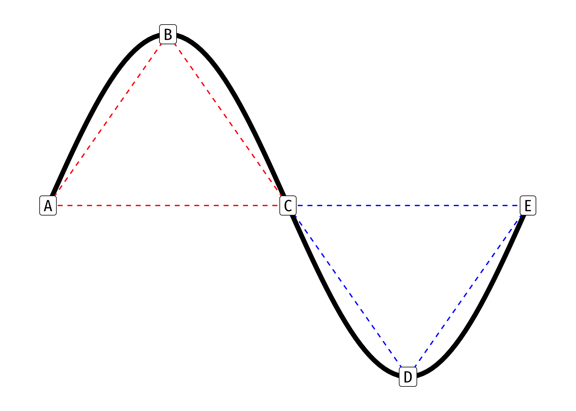
In simplest terms, a function is concave between two points \(a, b\) if a straight line connecting \(a\) and \(b\) lies beneath the function itself \[\color{red}{f[(t a)+(1-t)b]} > t f(a) + (1-t) f(b)\text{ for }0 < t < 1\]
- The above formula is a weighted average (for any set of weights \(w\), \(1-w\)), implying that the weighted average of \(a\) and \(b\) (dotted line in graph) is below the function
- The weighted average (dotted line) of \(a\) and \(b\) is below the function
- A function is also concave at a point if its second derivative at that point is negative \[\color{blue}{f[(w a)+(1-w)b]} < w f(a) + (1-w) f(b) \quad\text{ for }0 < w < 1\]
In simplest terms, a function is convex between two points \(a, b\) if a straight line connecting \(a\) and \(b\) lies above the function itself \[\color{blue}{f[(w a)+(1-w)b]} < w f(a) + (1-w) f(b) \quad \text{ for }0 < w < 1\] - The weighted average (dotted line) of \(a\) and \(b\) is above the function - A function is also convex at a point if its second derivative is positive
A function switches between convex and concave at an inflection point (point C in the example above) - Here, the second derivative (in addition to the first) is equal to 0
4.1 Optimization
For most curves, we often want to find the value where the function reaches its maximum or minimum (in general, these are types of “extrema”) along some interval
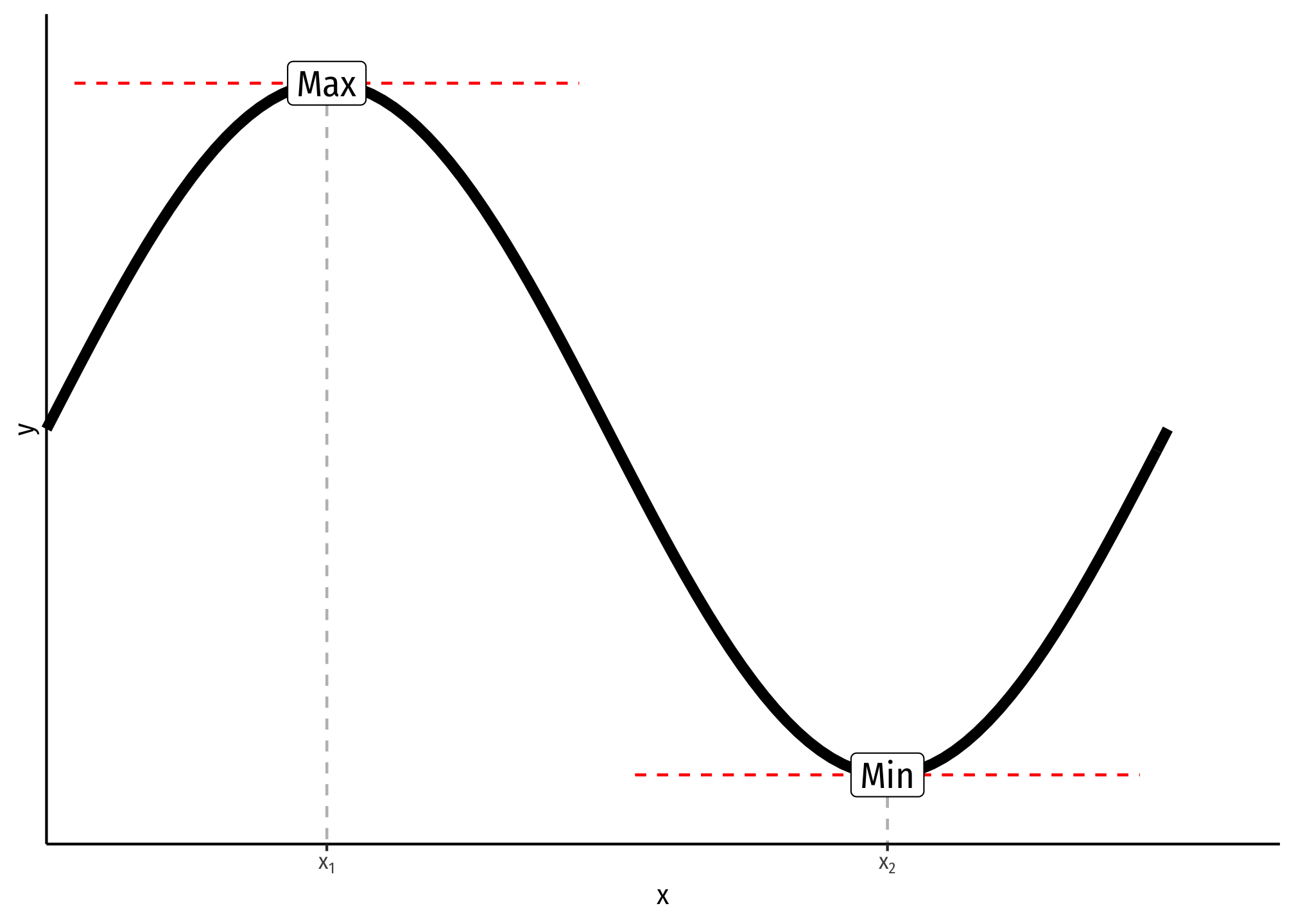
Formally, a function reaches a maximum at \(x^*\) if \(f(x^*) \geq f(x)\) for all \(x\); or a minimum at \(x^*\) if \(f(x^*) \leq f(x)\) for all \(x\) - In the graph above, the function reaches a maximum at \(x_1\) and a minimum at \(x_2\)
The maximum or minimum of a function occurs where the slope (first derivative) is zero, known in calculus as the “first-order condition” \[\frac{df(x^*)}{dx} = 0\]
- To distinguish between maxima and minima, we have the “second-order condition”
- A minimum occurs when the second derivative of the function is positive, and the curve is convex \[\frac{d^2f(x^*)}{dx^2} > 0\]
- A maximum occurs when the second derivative of the function is negative, and the curve is concave \[\frac{d^2f(x^*)}{dx^2} < 0\]
- An inflection point occurs where the second derivative of the function is zero
- All three are known as “critical points”
This is often useful for unconstrained optimization, e.g. finding the quantity of output that maximizes profits
Note, if we have a multivariate function \(y=f(x_1, x_2)\) and want to find the maximum or minimum (\(x_1^\star, x_2^\star\)), the first order conditions (FOC, plural) are where all the partial derivatives (derivative with respect to \(x_1\) and derivative with respect to \(x_2\)) are zero \[\begin{align*} \frac{\partial f(x_1^*, x_2^*)}{\partial x_1} &= 0 \\ \frac{\partial f(x_1^*, x_2^*)}{\partial x_2} &= 0 \\ \end{align*}\] There are second order conditions as well, to demonstrate whether an extremum is a maximum or minimum, but they are too complex to discuss here.
Often we want to find the maximum or minimum of a function over some restricted values of \((x_1, x_2)\), known as constrained optimization. This is one of the most important modeling tools in microeconomics, and will show up in many contexts.
- We want to find the maximum of some function:
\[
\begin{align*}
\max_{x_1, x_2} f(x_1, x_2)\\
\text{subject to } g(x_1, x_2)=c \\
\end{align*}
\]
- \(f(x_1, x_2)\) is the “objective function” we wish to maximize (or minimize)
- \(g(x_1, x_2)=c\) is the “constraint” that limits us within some specified set of \(x_1\) and \(x_2\) values
Much of microeconomic modeling is about figuring out what an agent’s objective is (e.g. maximize profits, maximize utility, minimize costs) and what their constraints are (e.g. budget, time, output).
There are several ways to solve a constrained optimization problem (see Appendix to Ch. 5 in textbook), the most frequent (but requiring calculus) is Lagrangian multiplier method.
Graphically, the solution to a constrained optimization problem is the point where a curve (objective function) and a line (constraint) are tangent to one another: they just touch, but do not intersect (e.g. at point A below).
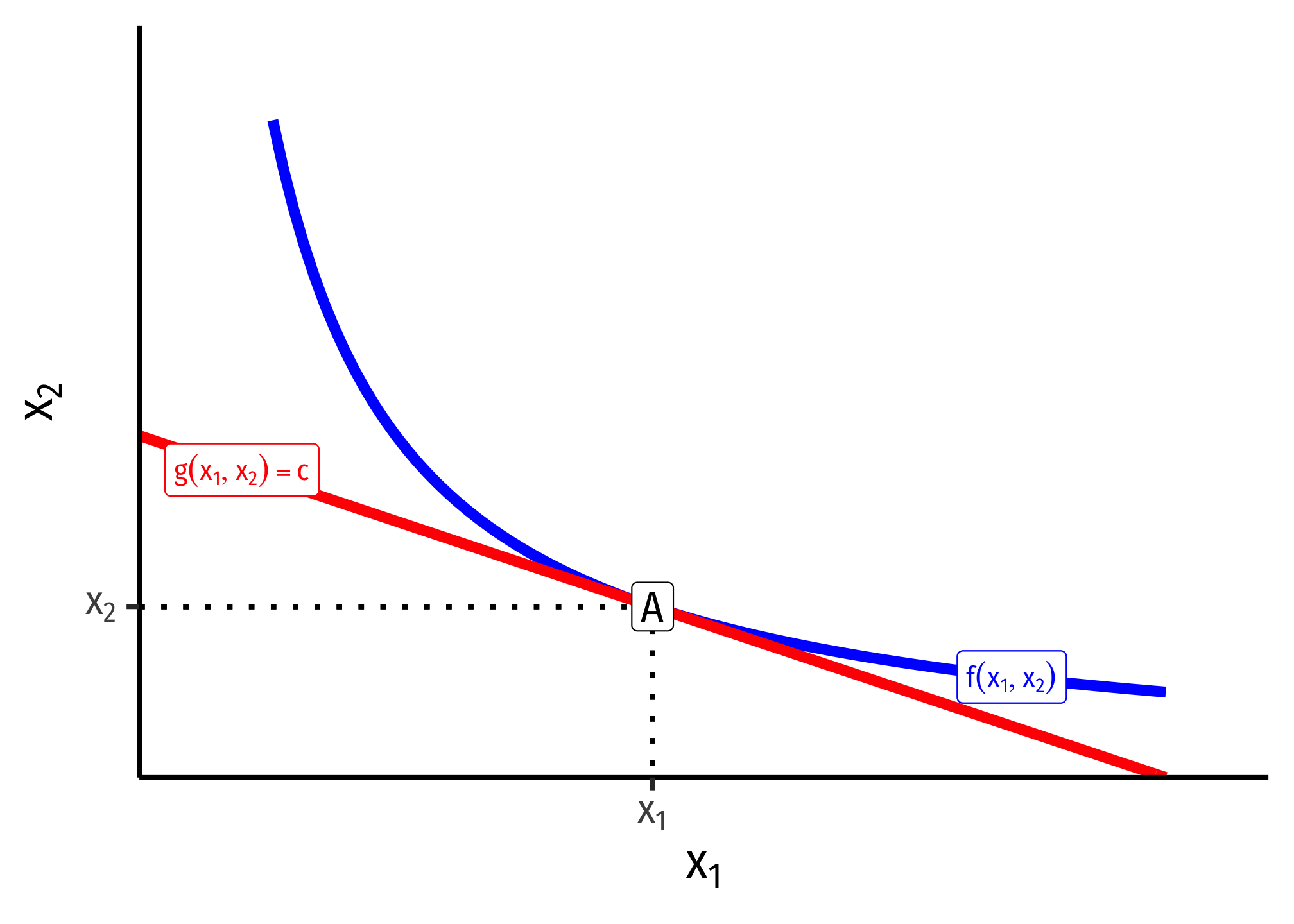
At the point of tangency (A), the slope of the curve (objective function) is equal to the slope of the line (constraint) - This is extremely useful and is always the solution to simple constrained optimization problems, e.g. - e.g. maximizing utility subject to income - e.g. minimizing cost subject to a certain level of output - We can find the equation of the tangent line using point slope form
\[y-y_1=m(x-x_1)\] - We need to know the slope \(m\), which we would know from the slope of the function at that point - We know \((x_1, y_1\)) is the point of tangency
5 Solving Systems of Equations
To solve a system of simultaneous linear equations, there must be as many equations as there are variables: \[ \begin{align*} 12x+4y&=36 \\ 6x-3y&=3 \\ \end{align*} \] There are two methods we can use to solve this system:
5.1 Substitution
First, we take one equation and solve for one of the variables. Here, we take the first, and solve for \(x\):
\[\begin{align*} 12x+4y&=36\\ 12x&=36-4y\\ x&=3-\frac{1}{3}y\\ \end{align*}\]
Now we take this value and plug it into the other equation:
\[\begin{align*} 6x-3y&=3\\ 6(3-\frac{1}{3}y)-3y&=3\\ 18-2y-3y&=3\\ 18-5y&=3\\ -5y&=-15\\ y&=3\\ \end{align*}\]
Now that we know the value of one variable, plug it into either of the original equations to solve for the value of the other variable:
\[ \begin{align*} 12x+4y&=36\\ 12x+4(3)&=36\\ 12x+12&=36\\ 12x&=24\\ x&=2\\ \end{align*} \]
We should verify that our variables are correct, so plug \(x\) and \(y\) into each equation and make sure it is true. Let’s start with the first equation:
\[\begin{align*} 12x+4y&=36\\ 12(2)+4(3)&=36\\ 24+12&=36 \checkmark \\ \end{align*}\]
We can do the same with the other equation:
\[\begin{align*} 6x-3y&=3\\ 6(2)-3(3)&=3\\ 12-9&=3 \checkmark \\ \end{align*}\]
5.2 Elimination
We will multiply the equations by constants to make the coefficients of one variable equal. Here, let us try to make the coefficients in front of each equation’s \(x\) equal.
\[\begin{align*} [12x+4y&=36]*6\\ [6x-3y&=3]*12\\ \end{align*}\]
To do so, we will multiply the first equation by 6, and the second equation by 12. (We multiply each equation by the coefficient in front of the other equation’s \(x\) variable):
\[\begin{align*} 72x+24y&=216\\ 72x-36y&=36 \end{align*}\]
Now we subtract the second equation from the first, which should get rid of \(x\):
\[\begin{align*} 72x+24y&=216\\ -[72x-36y&=36]\\ \end{align*}\]
Be careful to distribute the minus sign carefully:
\[\begin{align*} [72x-72x]+[24y-(-36y)]&=[216-36]\\ 60y&=180\\ y&=3\\ \end{align*}\]
Now that we have the value of one variable, plug it in to either equation.
\[\begin{align*} 12x+4y&=36\\ 12x+4(3)&=36\\ 12x+12&=36\\ 12x&=24\\ x&=2\\ \end{align*}\]
Now that we have both variables, we can plug them in to each equation to double check them, same as before.
6 Exponents and Logarithms
Exponents are defined as:
- \(b^n=\underbrace{b \times b \times ... \times b}_{n}\), where base \(b\) is multiplied by itself \(n\) times
- \(b^0=1\) (for \(b \neq 0\))
There are some common rules for exponents, assuming \(x\) and \(y\) are real numbers, \(m\) and \(n\) are integers, and \(a\) and \(b\) are rational:
- \(x^{-n}=\frac{1}{x^n}\)
- e.g. \(x^{-3} = \frac{1}{x^3}\)
- \(x^{\frac{1}{n}}=\sqrt[n]{x}\)
- e.g. \(x^{\frac{1}{2}} = \sqrt{x}\)
- \(x^{(\frac{m}{n})}=(x^{\frac{1}{n}})^m\)
- e.g. \(8^{\frac{4}{3}} = (8^\frac{1}{3})^4=2^4=16\)
- \(x^{a}x^b=x^{a+b}\)
- e.g. \(x^2x^3=x^5\)
- \(\frac{x^a}{x^b}=x^{a-b}\)
- e.g. \(\frac{x^2}{x^3}=x^{-1}=\frac{1}{x}\)
- \((\frac{x}{y})^a=\frac{x^a}{y^a}\)
- e.g. \((\frac{x}{y})^2=\frac{x^2}{y^2}\)
- \((xy)^a=x^ay^a\)
- e.g. \((xy)^2=x^2y^2\)
Logarithms are the exponents in the expressions above, the inverse of exponentiation
- If \(b^y=x\), then \(log_b(x)= y\)
- \(y\) is the number you must raise \(b\) to in order to get \(x\)
- e.g. \(2^6=64 = \underbrace{(2*2*2*2*2*2)}_{\text{6 times}}\) so \(log_2(64)=6\)
We often use the natural logarithm (ln) with base \(e=2.718...\) in many math, statistics, and economic applications
- If \(e^y=x\), then \(\ln(x) = y\)
There are a number of highly useful rules for natural logs:
- \(\ln(xy)=\ln(x)+\ln(y)\)
- e.g. \(\ln(2*3)=\ln(2)+\ln(3)\)
- \(\ln(\frac{x}{y})=\ln(x)-\ln(y)\)
- e.g. \(\ln(\frac{2}{3})=\ln(2)-\ln(3)\)
- \(\ln(x^a)=a*\ln(x)\)
- e.g. \(\ln(x^2)=2\ln(x)\)