Constrained Optimization I
We model most situations as a constrained optimization problem:
People optimize: make tradeoffs to achieve their objective as best as they can
Subject to constraints: limited resources (income, time, attention, etc)

Constrained Optimization II
One of the most generally useful mathematical models
Endless applications: how we model nearly every decision-maker
consumer, business firm, politician, judge, bureaucrat, voter, dictator, pirate, drug cartel, drug addict, parent, child, etc
- Key economic skill: recognizing how to apply the model to a situation
Remember!

Constrained Optimization III
- All constrained optimization models have three moving parts:
Constrained Optimization III
- All constrained optimization models have three moving parts:
- Choose: < some alternative >
Constrained Optimization III
- All constrained optimization models have three moving parts:
Choose: < some alternative >
In order to maximize: < some objective >
Constrained Optimization III
- All constrained optimization models have three moving parts:
Choose: < some alternative >
In order to maximize: < some objective >
Subject to: < some constraints >
Constrained Optimization: Example I
Example: A Hood student picking courses hoping to achieve the highest GPA while getting an Econ major.
Choose:
In order to maximize:
Subject to:

Constrained Optimization: Example II
Example: How should FedEx plan its delivery route?
Choose:
In order to maximize:
Subject to:
Constrained Optimization: Example III
Example: The U.S. government wants to remain economically competitive but reduce emissions by 25%.
Choose:
In order to maximize:
Subject to:

Constrained Optimization: Example IV
Example: How do elected officials make decisions in politics?
Choose:
In order to maximize:
Subject to:

The Utility Maximization Problem
- The individual's utility maximization problem we've been modeling, finally, is:
Choose: < a consumption bundle >
In order to maximize: < utility >
Subject to: < income and market prices >

The Utility Maximization Problem: Tools
We now have the tools to understand individual choices:
Budget constraint: individual’s constraints of income and market prices
- How market trades off between goods
- Marginal cost (of good , in terms of
Utility function: individual’s objective to maximize, based on their preferences
- How individual trades off between goods
- Marginal benefit (of good , in terms of

The Utility Maximization Problem: Verbally
- The individual's constrained optimization problem:
choose a bundle of goods to maximize utility, subject to income and market prices
The Utility Maximization Problem: Mathematically
- This requires calculus to solve.† We will look at graphs instead!
† See the mathematical appendix in today's class notes on how to solve it with calculus, and an example.
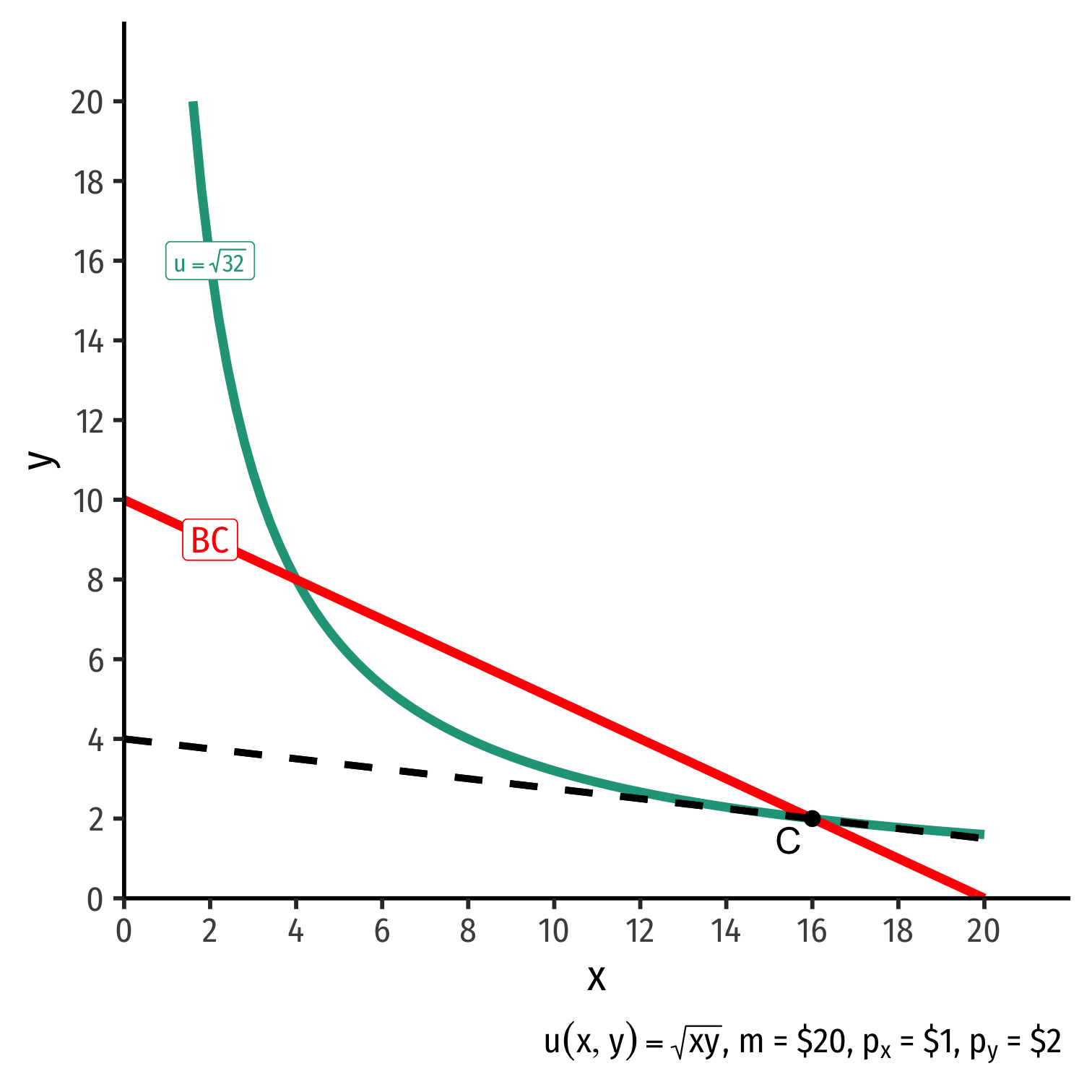
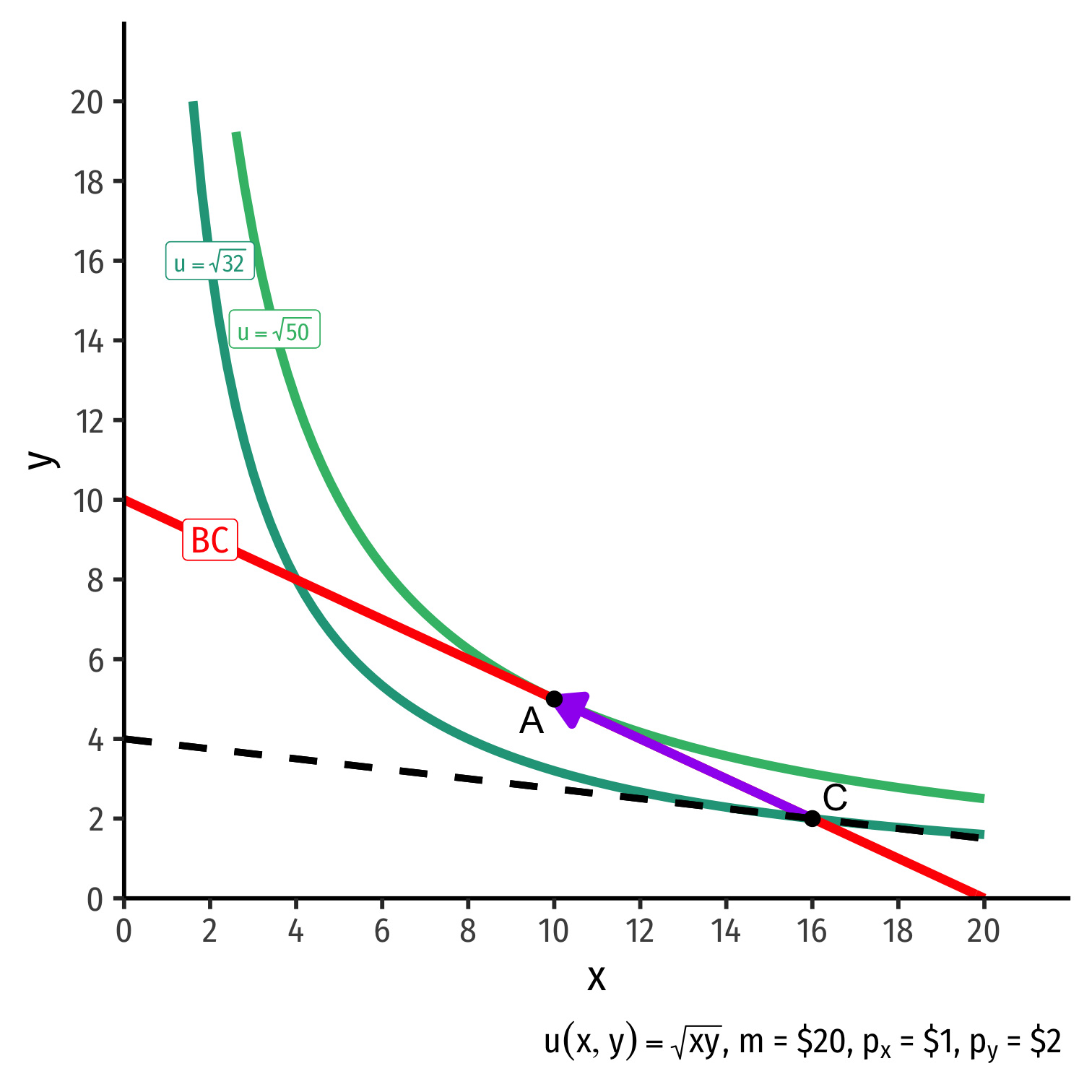
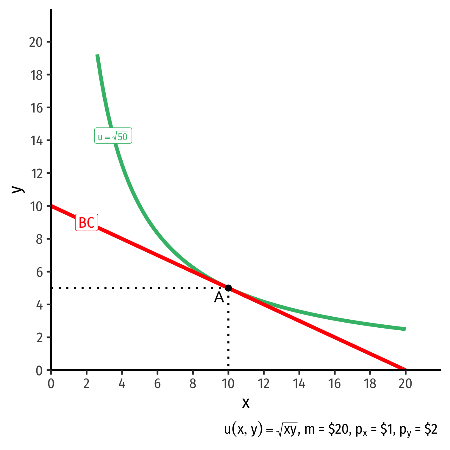
The Individual's Optimum: Graphically
- Graphical solution: Highest indifference curve tangent to budget constraint
- Bundle A!

The Individual's Optimum: Graphically
Graphical solution: Highest indifference curve tangent to budget constraint
- Bundle A!
B or C spend all income, but a better combination exists
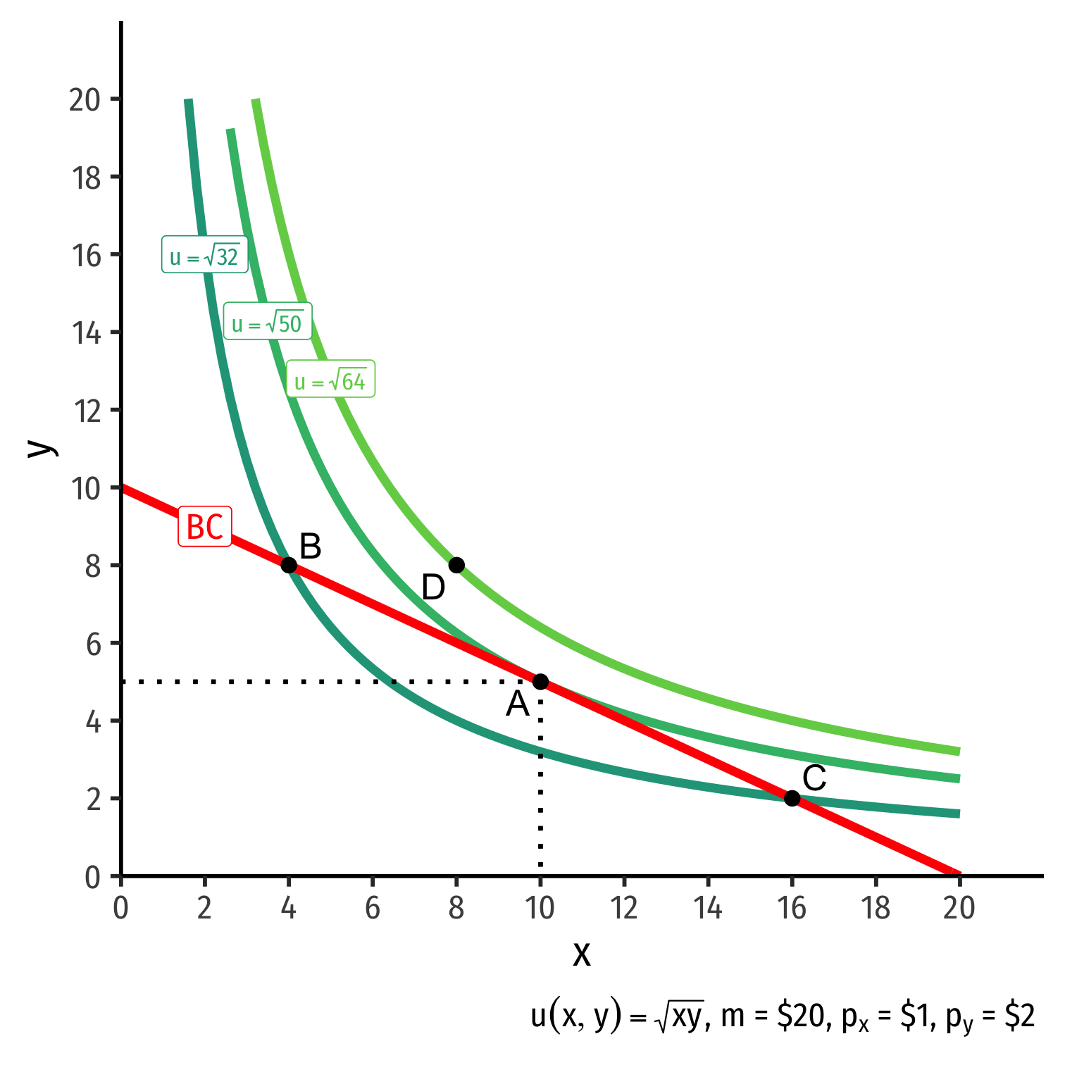
The Individual's Optimum: Graphically
Graphical solution: Highest indifference curve tangent to budget constraint
- Bundle A!
B or C spend all income, but a better combination exists
D is higher utility, but not affordable at current income & prices

The Individual's Optimum: Why Not B?

The Individual's Optimum: Why Not B?
Consumer views MB of is 2 units of
- Consumer’s “exchange rate:” 2Y:1X
Market-determined MC of is 0.5 units of
- Market exchange rate is 0.5Y:1X
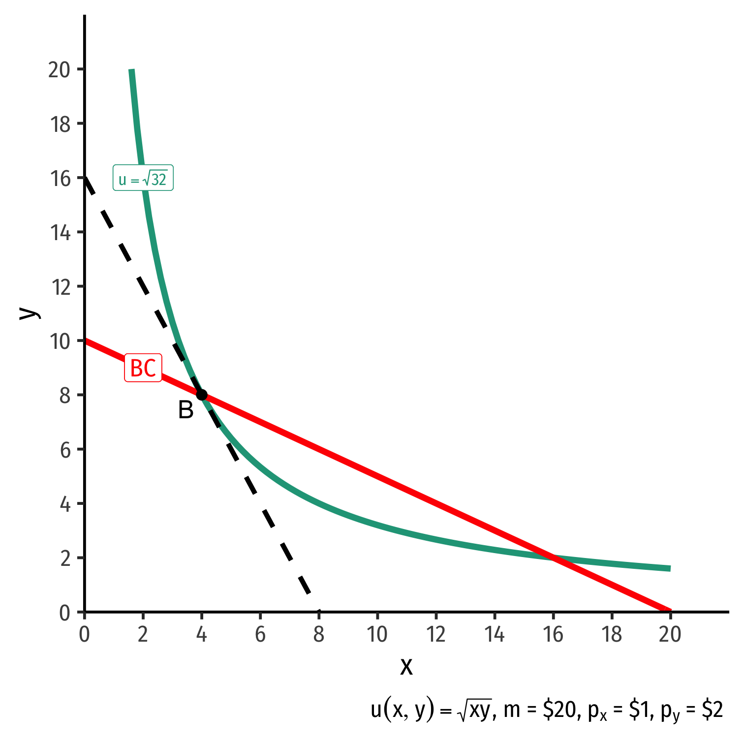
The Individual's Optimum: Why Not B?
Consumer views MB of is 2 units of
- Consumer’s “exchange rate:” 2Y:1X
Market-determined MC of is 0.5 units of
- Market exchange rate is 0.5Y:1X
Can spend less on y, more on x for more utility!
The Individual's Optimum: Why Not C?

The Individual's Optimum: Why Not C?
Consumer views MB of is 0.125 units of
- Consumer’s “exchange rate:” 0.125Y:1X
Market-determined MC of is 0.5 units of
- Market exchange rate is 0.5Y:1X
The Individual's Optimum: Why Not C?
Consumer views MB of is 0.125 units of
- Consumer’s “exchange rate:” 0.125Y:1X
Market-determined MC of is 0.5 units of
- Market exchange rate is 0.5Y:1X
Can spend less on y, more on x for more utility!
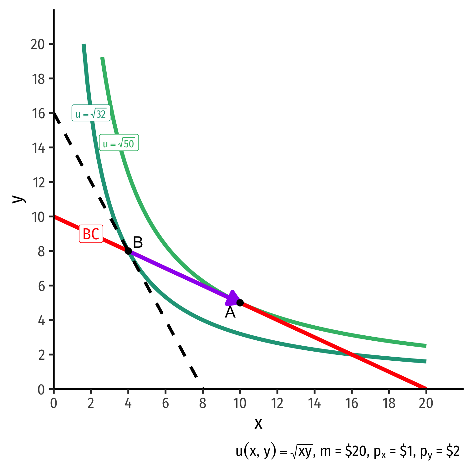
The Individual's Optimum: Why A?

The Individual's Optimum: Why A?
Marginal benefit = Marginal cost
- Consumer exchanges at same rate as market
No other combination of (x,y) exists that could increase utility!†
† At current income and market prices!
The Individual's Optimum: Two Equivalent Rules
Rule 1
- Easier for calculation (slopes)

The Individual's Optimum: Two Equivalent Rules
Rule 1
- Easier for calculation (slopes)
Rule 2
- Easier for intuition (next slide)

An Optimum, By Definition
Any optimum in economics: no better alternatives exist under current constraints
No possible change in your consumption that would increase your utility